Use Custom Time Scaling for a Rotation Trajectory
This example shows how to specify custom time-scaling in the Rotation Trajectory block to execute an interpolated trajectory. Two rotations are specified in the block to generate a trajectory between them. The goal is to move between rotations using a nonlinear time scaling with more time samples closer to the final rotation.
Specify the Time Scaling
Create vectors for the time scaling time vector and time scaling values. The time scaling time is linear vector from 0 to 5 seconds at 0.1 second intervals. The time scaling values follow a cubic trajectory with the appropriate derivatives specified for velocity and acceleration. These values are used in the model.
tsTime = 0:0.1:5;
tsVals(1,:) = (tsTime/5).^3;        % Position
tsVals(2,:) = ((3/125).*tsTime).^2;  % Velocity
tsVals(3,:) = (18/125^2).*tsTime;   % Acceleration
Open the Model
The Clock block outputs simulation time and is used for querying the rotation trajectory at those specify time points. The full set of time scaling time and values are input to the Rotation Trajectory block, but the Time input defined when to sample from this trajectory. The MATLAB® function block uses plotTransforms to plot a coordinate frame that moves along the generated rotation trajectory.
open_system("custom_time_scaling_rotation")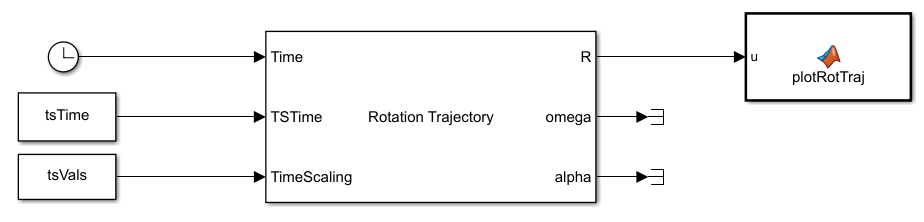
Simulate the Model
Simulate the model. The plot shows how the rotation follows a nonlinear interpolated trajectory parameterized in time. The model runs with a fixed-step solver at an interval of 0.1 seconds, so each frame is 0.1 seconds apart. Notice that the transformations are sampled more closely near the final rotation.
sim("custom_time_scaling_rotation")
hold off
