Motion Planning for Backhoe Using RRT

Since R2022b

This example shows how to plan a path for a backhoe, in an environment that contains obstacles, by using a motion planner. In this example, you model the backhoe in simplified form as a kinematic tree, then use a sampling-based motion planner to determine a viable path for the backhoe between two poses in the presence of obstacles. Simulate the outcome in a Simscape™ Multibody™ model.

Obtain Backhoe Model

This example uses a backhoe modeled in Simscape. The example builds off of the existing model in the Backhoe (Simscape Multibody) example, which simulates a backhoe under PID control. The model passes inputs from a set of reference trajectories to joints actuated by hydraulic pistons. The controller ensures that the joints reach the correct angles to execute the reference path.

This example modifies the model to accept trajectories from planned paths, and adds an obstacle to the workspace that represents a wall in the work area of the backhoe. The goal is to calculate a planned path to provide to the instrumented model so that it executes the collision-free trajectory.

open_system("sm_backhoe_with_environment")

Initialize runtime parameters for the initial trajectory values and the total length of the trajectory in seconds.

actPath = ones(4,60); % Initial Trajectory values
maxTime = 20;          % Length (s) of the planned trajectory

Create Model for Motion Planning

The original backhoe is a complex multi-domain model with many interconnected linkages. To efficiently plan a path for this system, you can create and use a simplified, tree-based representation of the backhoe instead. This simplified backhoe is a kinematic chain with four revolute joints, corresponding to the four PID-controlled angles in the associated Simulink® model. The simplified model must have these qualities:

• The kinematic tree structure must have the same dimensions as the original model.

• Joint limits must be consistent with the original model.

• Collision objects must conservatively estimate the bodies of the original model.

The kinematic tree must contain at least four joints, corresponding to the four actuated joints on the backhoe. A rotational joint to rotate the arm laterally, and three rotational joints that enable the backhoe to move the bucket vertically.

In the original backhoe, the loop closures from the hydraulic pistons limit the motion of these joints. However, these linkages do not exist in the simplified tree model, so you must apply joint limits directly using constraints.

The tree must have collision bodies that represent the elements that must not collide with obstacles. Here, these are modeled as prisms and cylinders that encompass all of the associated moving parts. Since the linkages have been simplified for planning purposes, the collision bodies are slightly oversized to ensure a conservative collision estimate during planning.

Start creating a tree that satisfies these requirements. First, directly import from the original Simscape model, then add the joint limits and collisions. For more details on this process, see the file for the helperImportAndCreateBackhoeRBT helper function.

[backhoeRBT,activeConfigIdx] = helperImportAndCreateBackhoeRBT;

Get the home configuration of the backhoe, and update it to set the controlled angles to nonzero values.

configToShow = homeConfiguration(backhoeRBT);
configToShow(activeConfigIdx) = [0 -pi/4 pi/12 -pi/24];

Visualize the results and adjust the view to fit.

ax = show(backhoeRBT,configToShow,Collisions="on"); 
title("Imported Rigid Body Tree with Collisions")
xlim([-8.5 14.5])
ylim([-17 6.5])
zlim([-11 12])
ax.Position = [0.1300 0.1100 0.7750 0.7150];
view(-60,27.5)

Create Motion Planner

Now that you have modeled the robot, you can create the motion planner. The planner accepts the rigid body tree, representing the backhoe, and a cell array of collision objects, representing the environment. To demonstrate the motion planner, the environment must contain a wall as a collision box.

Create the collision box, add it to the environment cell array, and change its position.

env = {collisionBox(.5,10,5)};
env{1}.Pose = trvec2tform([0 -17 -2]);

Create the motion planner. Use the manipulatorRRT object, which is designed to plan motion for robots with a tree-like structure.

planner = manipulatorRRT(backhoeRBT,env);

Next, configure the planner. Scale the connection distance and validation distance to the task. Determining these values requires some trial and error.

planner.MaxConnectionDistance = 1;
planner.ValidationDistance = 0.03;

Because the moving parts of the rigid body tree are relatively simple, and its motion is already constrained by joint limits, self-collision is unlikely. In this case, you can potentially increase the efficiency of the planner by eliminating self-collision checks. Set the planner to ignore self-collisions.

planner.IgnoreSelfCollision = true;
planner.SkippedSelfCollisions = "parent"; % Set parameter explicitly to avoid compatibility warning

Set Up Planning Problem

Define the start and goal poses. The planner attempts to find a collision-free path between these two poses.

% Set initial and final position targets, using the active configuration
% index to ensure only controlled joints are set (other values are
% arbitrary)
initialState = [pi/8 -pi/4 0 0];
qStart = backhoeRBT.homeConfiguration;
qStart(activeConfigIdx) = initialState;

targetState = [-pi/8 -pi/12 -pi/4 0];
qGoal = backhoeRBT.homeConfiguration;
qGoal(activeConfigIdx) = targetState;

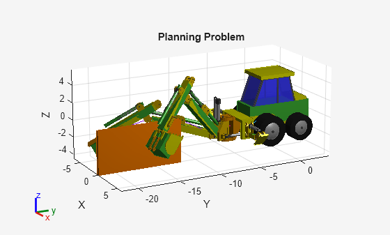
Visualize the environment and the start and the goal poses of the backhoe.

figure
ax = show(backhoeRBT,qStart,Collisions="on");
title("Planning Problem")
hold on
show(backhoeRBT,qGoal,Collisions="on",PreservePlot=true,Parent=ax); 
show(env{1},Parent=ax);
view(62,16)
axis equal
hold off

Plan Collision-Free Path

Set the random seed, for repeatability, and then run the planner to compute a collision-free path.

rng(20); % For repeatability
path = plan(planner,qStart',qGoal');

Because of the design of the planner, the initial returned path may be inefficient and appear somewhat random. Use the shorten routine to iterate on the path and find a more optimized solution. Then smooth the results by interpolating between the planned poses.

shortenedPath = shorten(planner,path,20);
smoothPath = interpolate(planner,shortenedPath,5);

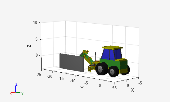
Visualize the planned path in MATLAB®. This output shows the outcome of the planner using the simplified model and environment.

figure
ax = show(backhoeRBT,qStart,Collisions="on");
xlim([-5 5])
ylim([-25 5])
zlim([-4 10])
drawnow
hold on
show(env{1},Parent=ax);
pause(0.5)
rc = rateControl(10);
for i = 1:size(smoothPath,1)
    show(backhoeRBT,smoothPath(i,:)',Parent=ax,Collisions="on",FastUpdate=true,PreservePlot=false);
    waitfor(rc);
end
hold off

Simulate Planned Path in Simulink

Return to the Simulink model and execute it using the sampled, planned path as input. Since Simulink simulates the model over time, you must convert the sampled path to a smooth trajectory. You can do so by using the Minimum Jerk Polynomial Trajectory block.

The resulting model produces a collision-free trajectory that you can execute with the existing backhoe model.

% Get the waypoints for the actuators & provide them to the model
actPath = smoothPath(:,activeConfigIdx)';

% Suppress benign warnings
mutedWarnings = helperMuteBenignWarnings();
for i = 1:numel(mutedWarnings)
    restoreWarnings{i} = onCleanup(@()warning(mutedWarnings{i}));
end

open_system("sm_backhoe_with_environment")
sim("sm_backhoe_with_environment")

% Clear the warning object
clear restoreWarnings;

Possible Variations and Extensions

In this example, you have planned a collision-free path for a complex system by modeling the system as a tree and planning a path for that tree. You then executed the planned path in Simulink as a single, continuous trajectory provided to controlled joint angles.

Use Planner That Allows Greater Fidelity System Modeling

The approach in this example is efficient because the system it models can be modeled as a tree without a significant loss of accuracy. This enables the motion planner to compute forward kinematics without incorporating kinematic constraints, which are computationally expensive. Using the tree also enables you to use a motion planner. However, for systems that require greater fidelity, you might need to model the complete system with kinematic constraints. In that case, use a planner that allows for general system models.

The manipulatorStateSpace and the manipulatorCollisionBodyValidator objects provide interfaces that enable users to plan paths for constrained rigid body tree objects. For more information about constrained path planning, see Plan Paths with End-Effector Constraints Using State Spaces for Manipulators. These objects enable you to enforce kinematic constraints with generalized inverse kinematics, which results in a more complex planner configuration. This complexity can be important for complex systems, or for systems for tight environments.

Smooth Trajectory Prior to Implementation in Simulink

In this example, the planned geometric path is scaled to Simulink by providing the path directly to a trajectory generator. However, the resulting trajectory is not quite as smooth as it could be. You can further smooth the trajectory by iterating over it using the shorten and interpolate functions. Additionally, you can resample the output path at a lower rate to produce a smoother trajectory. You can use these smoothing processes when the environment is minimally crowded, or when the collisions are conservatively estimated.