Rational Fit S-Parameters

This example shows how to use the rational object to create a rational fit to S-parameter data, and the various properties and methods that are included in the rational object.

Create Rational Object

Read in the sparameters, and create the rational object from them. The rational function automatically fits all entries of the S-parameter matrices.

S = sparameters('sawfilter.s2p')

S = 
  sparameters with properties:

      Impedance: 50
       NumPorts: 2
     Parameters: [2×2×334 double]
    Frequencies: [334×1 double]

r = rational(S)

r = 
  rational with properties:

      NumPorts: 2
      NumPoles: 24
         Poles: [24×1 double]
      Residues: [2×2×24 double]
    DirectTerm: [2×2 double]
         ErrDB: -40.9658

With the default settings on this example, the rational object achieves an accuracy of about -26 dB, using 30 poles. By construction, the rational object is causal, with a non-zero direct term.

Compare Fit with Original Data

Generate the frequency response from the rational object, and compare one of the entries with the original data.

resp = freqresp(r, S.Frequencies);
plot(S.Frequencies, real(rfparam(S, 1, 1)), ...
    S.Frequencies, real(squeeze(resp(1,1,:))))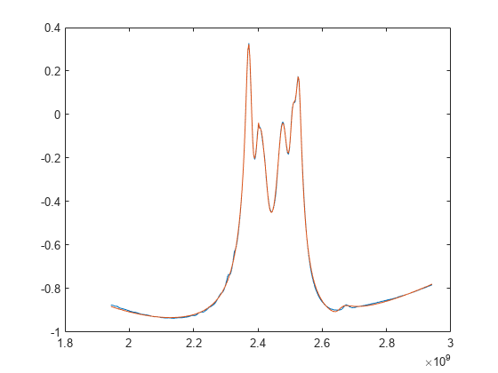

Limit Number of Poles

Redo the fit, limiting the number of poles to a maximum of 5. The rational object may use fewer poles than specified. Notice that the quality of the fit is degraded as opposed to the original 30-pole fit.

r5 = rational(S, 'MaxPoles', 5)

r5 = 
  rational with properties:

      NumPorts: 2
      NumPoles: 4
         Poles: [4×1 double]
      Residues: [2×2×4 double]
    DirectTerm: [2×2 double]
         ErrDB: -1.7376

resp5 = freqresp(r5, S.Frequencies);
plot(S.Frequencies, real(rfparam(S, 1, 1)), ...
    S.Frequencies, real(squeeze(resp5(1,1,:))))

Tighten Target Accuracy

Redo the fit, asking for a tighter tolerance (-60 dB), Notice that the fit is significantly improved, particularly in the stopbands of the SAW filter.

rgood = rational(S, -60,'QLimit',inf,'TendsToZero',false)

rgood = 
  rational with properties:

      NumPorts: 2
      NumPoles: 85
         Poles: [85×1 double]
      Residues: [2×2×85 double]
    DirectTerm: [2×2 double]
         ErrDB: -56.2635

respgood = freqresp(rgood, S.Frequencies);
plot(S.Frequencies, real(rfparam(S, 1, 1)), ...
    S.Frequencies, real(squeeze(respgood(1,1,:))))