Industrial Cooling Fan Anomaly Detection Algorithm Development for Deployment to a Microservice Docker Image
Detection of anomalies from sensor measurements is an important part of an equipment condition monitoring process for preventing catastrophic failure. This example shows the first part of a two-part end-to-end workflow for creating a predictive maintenance application from the development of a machine learning algorithm that can ultimately be deployed as a trained machine learning model in a Docker® microservice.
The example uses a Simulink® model to synthetically create measurement data for both normal and anomalous conditions. A support vector machine (SVM) model is trained for detecting anomalies in load, fan mechanics, and power consumption of an industrial cooling fan. The model detects a load anomaly when the system is working on overloaded conditions, that is, when the system work demand exceeds designed limits. A fan anomaly is detected when a fault occurs within the mechanical subsystem of the motor or the fan. Finally, a power supply anomaly can be detected by a drop in the voltage.
The companion example, Deploy Industrial Cooling Fan Anomaly Detection Algorithm as Microservice (MATLAB Compiler SDK), shows the actual deployment of the model in a Docker environment.
Data Generation
In this example, a thermistor-controlled fan model defined using Simscape™ Electrical™ blocks, generates the measurements. This Simulink model includes thermal, mechanical and electrical components of a fan. You can learn more about this model in Thermistor-Controlled Fan (Simscape Electrical).
addpath('Data_Generator/', 'Data_Generator/VaryingConvectionLib/');
mdl = "CoolingFanWithFaults";
open_system(mdl)
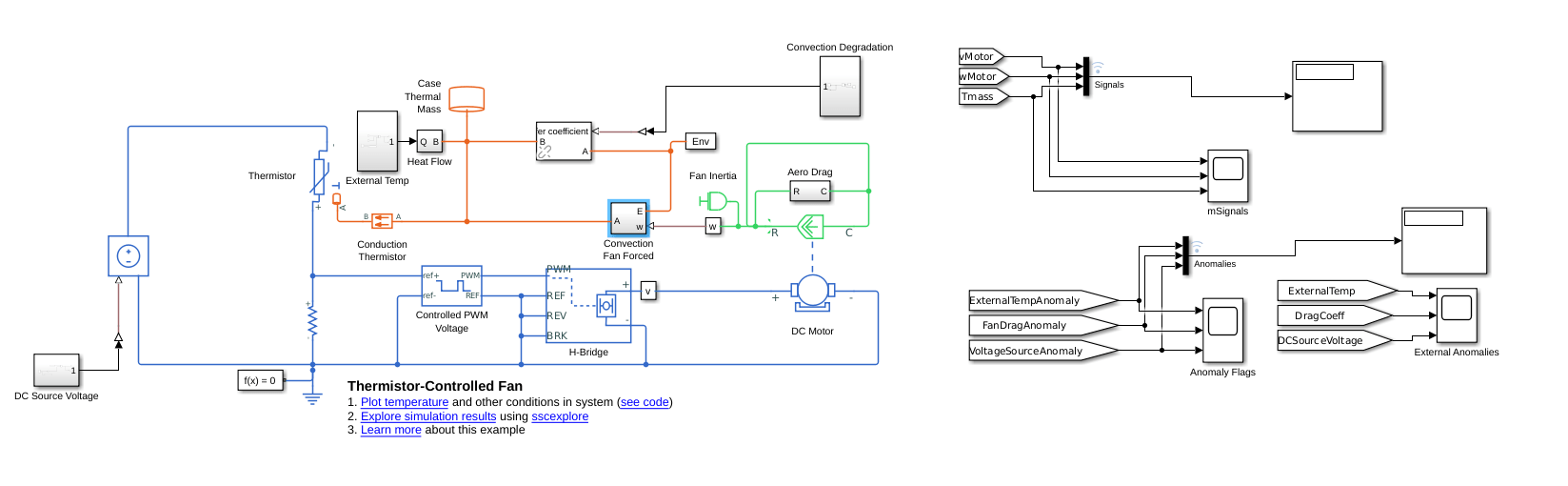
Anomalies are introduced to this model at random times and for random durations by using custom MATLAB® functions within the DC Source Voltage, Aero Drag and External Temp blocks. There are only three sensors located in this model: a voltage sensor, power sensor and temperature sensor. Data from these sensors is used to detect anomalies.
To generate data with sufficient instances of all anomalies, simulate the model 40 times with randomly generated anomalies. Note that these anomalies can occur in more than one component. The generateData helper function supports the simulation of the data. Within the generateData function, nominal ranges and the anomalous range are defined. The generateSimulationEnsemble function is used within generateData function to run the simulations, in parallel if Parallel Computing Toolbox has been installed, and generate the data for this experiment.
generateFlag = false;
if isfolder('./Data')
    folderContent = dir('Data/CoolingFan*.mat');
    if isempty(folderContent)
        generateFlag = true;
    else
        numSim = numel(folderContent);
    end
else
    generateFlag = true;
end

if generateFlag
    numSim = 40;
    rng("default");
    generateData('training', numSim);
end
Starting parallel pool (parpool) using the 'Processes' profile ...
16-Jan-2024 15:36:35: Job Queued. Waiting for parallel pool job with ID 3 to start ...
16-Jan-2024 15:37:36: Connected to 5 of 6 parallel pool workers.
Connected to parallel pool with 6 workers.
Once the simulations have been completed, load the data by using simulationEnsembleDatastore and set the selected variables to be Signals and Anomalies. SimulationEnsembleDatastore is a datastore specialized for use in developing algorithms for condition monitoring and predictive maintenance using simulated data. Create a simulation ensemble datastore for the data generated by the 40 simulations and set the selected variables appropriately.
ensemble = simulationEnsembleDatastore('./Data')ensemble =
simulationEnsembleDatastore with properties:
DataVariables: [4×1 string]
IndependentVariables: [0×0 string]
ConditionVariables: [0×0 string]
SelectedVariables: [4×1 string]
ReadSize: 1
NumMembers: 40
LastMemberRead: [0×0 string]
Files: [40×1 string]
ensemble.SelectedVariables = ["Signals", "Anomalies"];
Data Characteristics
Split the ensemble into training, test and validation subsets. Assign the first 37 members of the ensemble as the training set, next two members as the test set and the last member as the validation set. To visualize the signal characteristics, read the first member of the training ensemble and plot the signals and the anomaly labels associated with the measured signals.
trainEnsemble = subset(ensemble, 1:numSim-3)
trainEnsemble =
  simulationEnsembleDatastore with properties:

           DataVariables: [4×1 string]
    IndependentVariables: [0×0 string]
      ConditionVariables: [0×0 string]
       SelectedVariables: [2×1 string]
                ReadSize: 1
              NumMembers: 37
          LastMemberRead: [0×0 string]
                   Files: [37×1 string]
testEnsemble = subset(ensemble, numSim-2:numSim-1);
validationEnsemble = subset(ensemble, numSim);

tempData = trainEnsemble.read;
signal_data = tempData.Signals{1};
anomaly_data = tempData.Anomalies{1};

h = figure;
tiledlayout("vertical");
ax1 = nexttile; plot(signal_data.Data(:,1)); title('Motor Voltage')
ax2 = nexttile; plot(signal_data.Data(:,2)); title('Fan Speed')
ax3 = nexttile; plot(signal_data.Data(:,3)); title('Temperature'); xlabel('Time in seconds');
ax4 = nexttile; plot(anomaly_data.Data(:,1), 'bx', 'MarkerIndices',find(anomaly_data.Data(:,1)>0.1), 'MarkerSize', 5); hold on;
plot(anomaly_data.Data(:,2), 'ro', 'MarkerIndices',find(anomaly_data.Data(:,2)>0.1), 'MarkerSize', 5);
plot(anomaly_data.Data(:,3), 'square', 'Color', 'g', 'MarkerIndices',find(anomaly_data.Data(:,3)>0.1), 'MarkerSize', 5);
linkaxes([ax1 ax2 ax3 ax4],'x')
ylim([0, 2]);
title('Anomalies');
legend("Load Anomaly", "Fan Anomaly", "Power Supply Anomaly", 'Location', 'bestoutside')
set(h,'Units','normalized','Position',[0 0 1 .8]);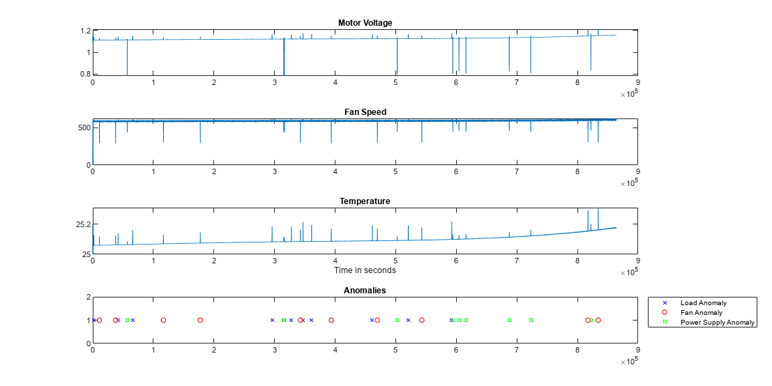
Anomalies are manifested as small pulses on the traces that last between 10 and 100 seconds. Notice that different types of anomalies have different profiles. The information contained in only one of these traces is not sufficient to classify among the different type of anomalies, as one anomaly can be manifested in more than one of the signals. Zoom in to see the signal characteristics when the anomalies occur. At this scale, it is clear that the magnitude of the raw measurements do change during periods of anomalies. The plot shows that more than one anomaly can occur at a time. Therefore, the anomaly detection algorithm needs to use the information in all three measurements to distinguish among anomalies in load, fan speed and power supply.
Model Development
Characteristics of the measured data and the possible anomalies are important in determining the modeling approach. As seen in the data above, anomalies can span multiple consecutive time steps. It is not sufficient to monitor just one signal. All three signals need to be monitored to identify each of the three anomalies. Furthermore, the selected model must have a quick response time. Therefore, the model needs to detect anomalies in reasonably small window size of data. Based on these factors and knowledge of the mechanical components, define a window size of 2000 time samples. This window size is sufficient to capture an anomalous event but at the same time is short enough for the anomaly detection to be quick.
The next step is to understand the balance of the dataset for the different anomaly cases. There are a total of eight different possibilities ranging from no anomalies in either load, fan speed or power supply, or anomalies in all three. Read in the trainingData and summarize the number of instances of each anomaly type. Single anomalies are represented as 'Anomaly1', two simultaneously occurring anomalies are labeled as 'Anomaly12' and anomalies in all three categories are labeled as 'Anomaly123'.
trainingData = trainEnsemble.readall;
anomaly_data = vertcat(trainingData.Anomalies{:});
labelArray={'Normal','Anomaly1','Anomaly2', 'Anomaly3', 'Anomaly12','Anomaly13','Anomaly23','Anomaly123'}';
yCategoricalTrain=labelArray(sum(anomaly_data.Data.*2.^(size(anomaly_data.Data,2)-1:-1:0),2)+1,1);
yCategoricalTrain=categorical(yCategoricalTrain);
summary(yCategoricalTrain);
Anomaly1 50653
Anomaly12 51123
Anomaly13 59
Anomaly2 48466
Anomaly23 64
Anomaly3 28
Normal 31817644
As seen above, the dataset is highly imbalanced. There are significantly more points for the normal condition than for anomalous conditions. The categories with multiple simultaneous anomalies occur even less frequently. To use the information in the multiple simultaneous anomaly cases (Anomaly12, Anomaly13, Anomaly23), train three independent classifiers. Each SVM model learns about only a single anomaly type. SVM looks at the interactions between the features and does not assume independence, as long as a non-linear kernel is used.
Features need to be extracted from raw measurement data to achieve a robust and well-performing model. The Diagnostic Feature Designer (DFD) app assists in the design of features. Create data ensembles using the makeEnsembleTableSimpleFrame helper function to represent the raw data as inputs to the DFD app. The helper function splits the time series into frames of size 2000 samples. To deal with the highly imbalanced nature of the dataset, use the downsampleNormalData helper function to reduce the number of frames with the normal label by about 87%. Use this reduced dataset in the DFD app to design features. For each anomaly type, import the data into the app and extract suitable features. Select the top ranked features to train the SVM. To reproduce the workflow, a MATLAB function diagnosticFeatures is instead exported from the DFD app and top features for all three anomaly types have been selected to compute a total of 18 features. Set startApp to true to instead open the DFD app and compute new features.
yTrainAnomaly1=logical(anomaly_data.Data(:,1));
yTrainAnomaly2=logical(anomaly_data.Data(:,2));
yTrainAnomaly3=logical(anomaly_data.Data(:,3));

windowSize=2000;
sensorDataTrain = vertcat(trainingData.Signals{:});
ensembleTableTrain1 = generateEnsembleTable(sensorDataTrain.Data,yTrainAnomaly1,windowSize);
ensembleTableTrain2 = generateEnsembleTable(sensorDataTrain.Data,yTrainAnomaly2,windowSize);
ensembleTableTrain3 = generateEnsembleTable(sensorDataTrain.Data,yTrainAnomaly3,windowSize);

ensembleTableTrain1_reduced = downsampleNormalData(ensembleTableTrain1);
ensembleTableTrain2_reduced = downsampleNormalData(ensembleTableTrain2);
ensembleTableTrain3_reduced = downsampleNormalData(ensembleTableTrain3);

startApp = false;
if startApp
    diagnosticFeatureDesigner; %#ok<UNRCH>
end

featureTableTrain1 = diagnosticFeatures(ensembleTableTrain1_reduced);
featureTableTrain2 = diagnosticFeatures(ensembleTableTrain2_reduced);
featureTableTrain3 = diagnosticFeatures(ensembleTableTrain3_reduced);

head(featureTableTrain1);
Anomaly Signal_tsmodel/Coef1 Signal_tsmodel/Coef2 Signal_tsmodel/Coef3 Signal_tsmodel/AIC Signal_tsmodel/Freq1 Signal_tsmodel/Mean Signal_tsmodel/RMS Signal_tsmodel_1/Freq1 Signal_tsmodel_1/Mean Signal_tsmodel_1/RMS Signal_tsfeat/ACF1 Signal_tsfeat/PACF1 Signal_tsmodel_2/Freq1 Signal_tsmodel_2/AIC Signal_tsmodel_2/Mean Signal_tsmodel_2/RMS Signal_tsfeat_2/ACF1 Signal_tsfeat_2/PACF1
_______ ____________________ ____________________ ____________________ __________________ ____________________ ___________________ __________________ ______________________ _____________________ ____________________ __________________ ___________________ ______________________ ____________________ _____________________ ____________________ ____________________ _____________________
true -0.9242 0.16609 -0.11822 -12.792 0.0025644 0.026824 0.03654 0.033299 109.08 109.14 0.95851 0.95851 0.0028621 -10.778 0.69223 0.89283 0.95851 0.95851
false -1.3919 0.81975 -0.44229 -20.091 0.033729 0.14008 0.14259 0.037706 124.55 124.99 0.86983 0.86983 0.040064 -17.217 3.8916 3.9242 0.86983 0.86983
true -1.0321 0.03862 -0.00024365 -13.944 0.0015275 0.010568 0.026864 0.018114 74.674 75.627 0.99134 0.99134 0.0015462 -12.103 0.2407 0.60553 0.99134 0.99134
false -1.4498 0.91956 -0.51851 -19.926 0.035592 0.13954 0.14229 0.050092 131.32 131.75 0.87307 0.87307 0.048074 -17.108 3.9129 3.9472 0.87307 0.87307
true -1.0293 0.033209 0.0083011 -13.533 0.0012723 0.0090939 0.026377 0.012409 53.697 55.074 0.99252 0.99252 0.0012741 -11.703 0.20546 0.59311 0.99252 0.99252
false -1.4505 0.90191 -0.50622 -19.87 0.037046 0.13092 0.13384 0.048943 122.97 123.44 0.8842 0.8842 0.059194 -17.086 3.6446 3.6818 0.8842 0.8842
false -1.4161 0.84038 -0.45416 -19.709 0.033386 0.13425 0.13696 0.040977 126.66 127.1 0.87985 0.87985 0.04078 -16.981 3.6891 3.7249 0.87985 0.87985
false -1.4301 0.87033 -0.47744 -19.628 0.023078 0.11943 0.1226 0.029963 114.56 115.07 0.88308 0.88308 0.02668 -16.915 3.2854 3.3272 0.88308 0.88308
Once the feature tables, which contain the features and the labels, have been computed for each anomaly type, train an SVM model with a gaussian kernel. Further, as seen in summary of one of the feature tables, the features have different ranges. To prevent the SVM model from being biased towards features with larger values, set the Standardize parameter to true. Save the three models to the anomalyDetectionModelSVM.mat file for use in a later section.
m.m1 = fitcsvm(featureTableTrain1, 'Anomaly', 'Standardize',true, 'KernelFunction','gaussian');
m.m2 = fitcsvm(featureTableTrain2, 'Anomaly', 'Standardize',true, 'KernelFunction','gaussian');
m.m3 = fitcsvm(featureTableTrain3, 'Anomaly', 'Standardize',true, 'KernelFunction','gaussian');

% Save model for reuse later
save anomalyDetectionModelSVM m
Model Testing and Validation
To test the model accuracy, use the data in the testEnsemble. Read the signal and anomaly data in testEnsemble, and from that data, create a data ensemble using the generateEnsembleTable helper function. Then, use the diagnosticFeatures function to compute the selected features.
testData = testEnsemble.readall;
anomaly_data_test = vertcat(testData.Anomalies{:});

yTestAnomaly1=logical(anomaly_data_test.Data(:,1));
yTestAnomaly2=logical(anomaly_data_test.Data(:,2));
yTestAnomaly3=logical(anomaly_data_test.Data(:,3));

sensorDataTest = vertcat(testData.Signals{:});
ensembleTableTest1 = generateEnsembleTable(sensorDataTest.Data,yTestAnomaly1,windowSize);
ensembleTableTest2 = generateEnsembleTable(sensorDataTest.Data,yTestAnomaly2,windowSize);
ensembleTableTest3 = generateEnsembleTable(sensorDataTest.Data,yTestAnomaly3,windowSize);

featureTableTest1 = diagnosticFeatures(ensembleTableTest1);
featureTableTest2 = diagnosticFeatures(ensembleTableTest2);
featureTableTest3 = diagnosticFeatures(ensembleTableTest3);

% Predict
results1 = m.m1.predict(featureTableTest1(:, 2:end));
results2 = m.m2.predict(featureTableTest2(:, 2:end));
results3 = m.m3.predict(featureTableTest3(:, 2:end));
Compare the predictions from the three models for each anomaly type are compared to the true labels using a confusion chart.
% Combine predictions and create final vector to understand performance
yT = [featureTableTest1.Anomaly, featureTableTest2.Anomaly, featureTableTest3.Anomaly];
yCategoricalT = labelArray(sum(yT.*2.^(size(yT,2)-1:-1:0),2)+1,1);
yCategoricalT = categorical(yCategoricalT);

yHat = [results1, results2, results3];
yCategoricalTestHat=labelArray(sum(yHat.*2.^(size(yHat,2)-1:-1:0),2)+1,1);
yCategoricalTestHat=categorical(yCategoricalTestHat);

figure
confusionchart(yCategoricalT, yCategoricalTestHat)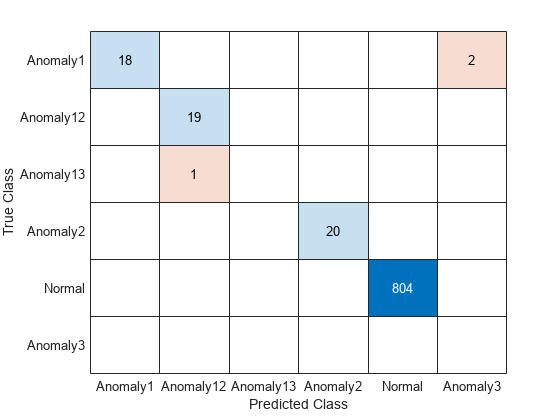
The confusion chart illustrates that the models performed well in identifying single and multiple simultaneous anomalies in the test data set. Since we are using three separate models, individual confusion charts can be created to visualize the performance of each model.
figure
tiledlayout(1,3);
nexttile; confusionchart(featureTableTest1.Anomaly, results1);
nexttile; confusionchart(featureTableTest2.Anomaly, results2);
nexttile; confusionchart(featureTableTest3.Anomaly, results3);

The confusion charts indicates that the models work well at identifying both single and multiple anomalies. At this point, a suitable model with satisfactory performance has been trained and tested. In the next section, repackage the algorithm to prepare it for deployment.
Deploy Anomaly Detection Algorithm Development as Microservice
You can now deploy the anomaly detection algorithm as a microservice which provides an HTTP/HTTPS endpoint to access the algorithm. For details, see the companion example Deploy Industrial Cooling Fan Anomaly Detection Algorithm as Microservice (MATLAB Compiler SDK).
You need MATLAB® Compiler SDK™ to execute the companion example.
See Also
Topics
- Deploy Industrial Cooling Fan Anomaly Detection Algorithm as Microservice (MATLAB Compiler SDK)
- Thermistor-Controlled Fan (Simscape Electrical)