Wave Equation on Square Domain: PDE Modeler App
This example shows how to solve a wave equation for transverse vibrations of a membrane on a square. The membrane is fixed at the left and right sides, and is free at the upper and lower sides. This example uses the PDE Modeler app. For a programmatic workflow, see Wave Equation on Square Domain.
A wave equation is a hyperbolic PDE:
To solve this problem in the PDE Modeler app, follow these steps:
Open the PDE Modeler app by using the
pdeModelercommand.Display grid lines by selecting Options > Grid.
Align new shapes to the grid lines by selecting Options > Snap.
Draw a square with the corners at (-1,-1), (-1,1), (1,1), and (1,-1). To do this, first click the
 button. Then click one of the corners using the right mouse
button and drag to draw a square. The right mouse button constrains the shape you
draw to be a square rather than a rectangle.
button. Then click one of the corners using the right mouse
button and drag to draw a square. The right mouse button constrains the shape you
draw to be a square rather than a rectangle.You also can use the
pderectfunction:pderect([-1 1 -1 1])
Check that the application mode is set to Generic Scalar.
Specify the boundary conditions. To do this, switch to boundary mode by clicking the
 button or selecting Boundary > Boundary Mode. Select the left and right boundaries. Then select Boundary > Specify Boundary Conditions and specify the Dirichlet boundary condition u = 0. This boundary condition is the default one (
h = 1,r = 0), so you do not need to change it.For the bottom and top boundaries, set the Neumann boundary condition ∂u/∂n = 0. To do this, set
g = 0,q = 0.Specify the coefficients by selecting PDE > PDE Specification or clicking the
 button on the toolbar. Select the
Hyperbolic type of PDE, and specify
button on the toolbar. Select the
Hyperbolic type of PDE, and specify c = 1,a = 0,f = 0, andd = 1.Initialize the mesh by selecting Mesh > Initialize Mesh. Refine the mesh by selecting Mesh > Refine Mesh.
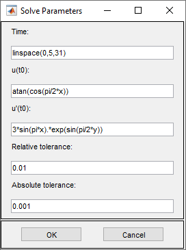
Set the solution times. To do this, select Solve > Parameters. Create linearly spaced time vector from 0 to 5 seconds by setting the solution time to
linspace(0,5,31).In the same dialog box, specify initial conditions for the wave equation. For a well-behaved solution, the initial values must match the boundary conditions. If the initial time is t = 0, then the following initial values that satisfy the boundary conditions:
atan(cos(pi/2*x))foru(0)and3*sin(pi*x).*exp(sin(pi/2*y))for ∂u/∂t,The inverse tangent function and exponential function introduce more modes into the solution.
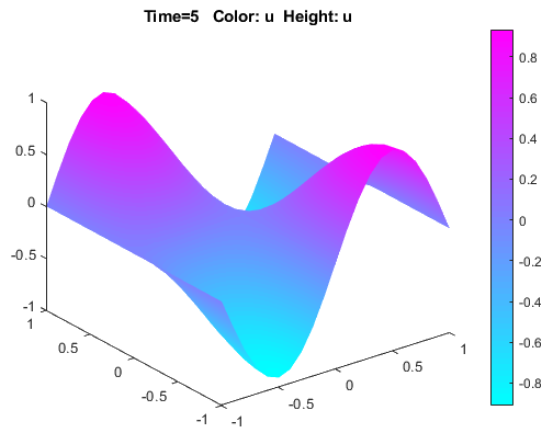
Solve the PDE by selecting Solve > Solve PDE or clicking the
 button on the toolbar. The app solves the heat
equation at times from 0 to 5 seconds and displays the result at the end of the time
span.
button on the toolbar. The app solves the heat
equation at times from 0 to 5 seconds and displays the result at the end of the time
span.Visualize the solution as a 3-D static and animated plots. To do this:
Select Plot > Parameters.
In the resulting dialog box, select the Color and Height (3-D plot) options.
To visualize the dynamic behavior of the wave, select Animation in the same dialog box. If the animation progress is too slow, select the Plot in x-y grid option. An x-y grid can speed up the animation process significantly.