Modal Superposition Method for Structural Dynamics Problem
This example shows how to solve a structural dynamics problem by using modal analysis results. Solve for the transient response at the center of a 3-D beam under a harmonic load on one of its corners. Compare the direct integration results with the results obtained by modal superposition.
Modal Analysis
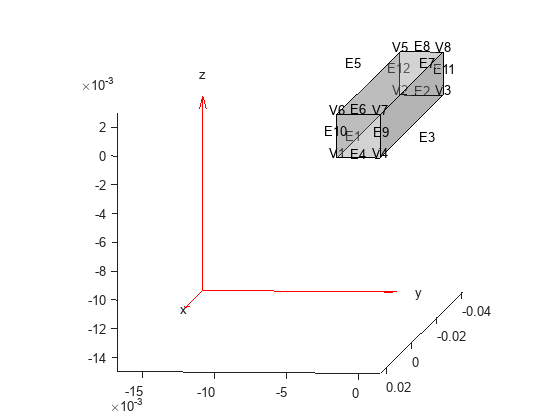
Create the geometry and plot it with the edge and vertex labels.
gm = multicuboid(0.05,0.003,0.003);
pdegplot(gm,EdgeLabels="on", ...
            VertexLabels="on", ...
            FaceAlpha=0.3);
view([95 5])
Create an femodel for modal structural analysis and include the geometry.
model = femodel(AnalysisType="structuralModal", ...
                 Geometry=gm);
Generate a mesh.
model = generateMesh(model);
Specify Young's modulus, Poisson's ratio, and the mass density of the material.
model.MaterialProperties = ...
    materialProperties(YoungsModulus=210E9, ...
                       PoissonsRatio=0.3, ...
                       MassDensity=7800);
Specify minimal constraints on one end of the beam to prevent rigid body modes. For example, specify that edge 4 and vertex 7 are fixed boundaries.
model.EdgeBC(4) = edgeBC(Constraint="fixed");
model.VertexBC(7) = vertexBC(Constraint="fixed");
Solve the problem for the frequency range from 0 to 500000. The recommended approach is to use a value that is slightly smaller than the expected lowest frequency. Thus, use -0.1 instead of 0.
Rm = solve(model,FrequencyRange=[-0.1,500000]);
Transient Analysis
Change the analysis type to transient structural.
model.AnalysisType = "StructuralTransient";Define a sinusoidal load function, sinusoidalLoad, to model a harmonic load. This function accepts the load magnitude (amplitude), the location and state structure arrays, frequency, and phase. Because the function depends on time, it must return a matrix of NaN of the correct size when state.time is NaN. Solvers check whether a problem is nonlinear or time-dependent by passing NaN state values and looking for returned NaN values.
function Tn = sinusoidalLoad(load,location,state,Frequency,Phase)
if isnan(state.time)
    Tn = NaN*[location.nx location.ny location.nz];
    return
end
if isa(load,"function_handle")
    load = load(location,state);
else
    load = load(:);
end
% Transient model excited with harmonic load
Tn = load.*sin(Frequency.*state.time + Phase);
end
Apply a sinusoidal force on the corner opposite the constrained edge and vertex.
Force=[0 0 10];
Frequency = 7600;
Phase = 0;
forcePulse = ...
    @(location,state) sinusoidalLoad(Force, ...
                                     location,state, ...
                                     Frequency,Phase);
model.VertexLoad(5) = vertexLoad(Force=forcePulse);
Specify the zero initial displacement and velocity.
model.CellIC = cellIC(Velocity=[0;0;0],Displacement=[0;0;0]);
Specify the relative and absolute tolerances for the solver.
model.SolverOptions.RelativeTolerance = 1E-5;
model.SolverOptions.AbsoluteTolerance = 1E-9;
Solve the model using the default direct integration method.
tlist = linspace(0,0.004,120);
Rd = solve(model,tlist);
Now, solve the model using the modal results.
tlist = linspace(0,0.004,120);
Rdm = solve(model,tlist,ModalResults=Rm);
Interpolate the displacement at the center of the beam.
intrpUd = interpolateDisplacement(Rd,0,0,0.0015);
intrpUdm = interpolateDisplacement(Rdm,0,0,0.0015);
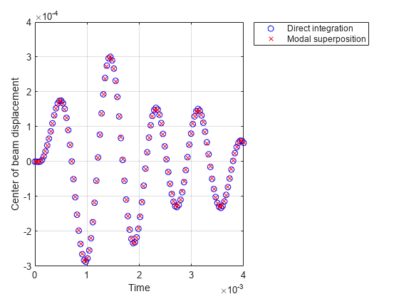
Compare the direct integration results with the results obtained by modal superposition.
plot(Rd.SolutionTimes,intrpUd.uz,"bo")
hold on
plot(Rdm.SolutionTimes,intrpUdm.uz,"rx")
grid on
legend("Direct integration", "Modal superposition")
xlabel("Time");
ylabel("Center of beam displacement")