Effect of Metastability Impairment in Flash ADC

Open Model

This example shows how to customize a flash Analog to Digital Converter (ADC) by adding the metastability probability as an impairment. You can measure the metastability probability impairment to validate your implementation. The example also shows the effect of metastability on the dynamic performance of the flash ADC. When the digital output from a comparator is ambiguous (neither zero nor one), the output is defined as metastable. The ambiguous output is expressed as NaN. This example model uses a MATLAB function block to add the metastability impairment to a flash ADC architecture. Another subsystem reports the metastability probability on the fly.

Customize Flash ADC

Extract the inner structure of the flash ADC to add customized impairment. Add a Flash ADC block from the Mixed-Signal Blockset™ library to a Simulink® canvas. Look under the mask to find the flat structure of the ADC. Copy and paste the complete structure to another new blank canvas.

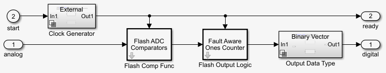
Delete the Clock Generator block because it is not used to provide the start conversion clock. An external Stimuli subsystem is used for that purpose. The flash ADC now consists of three major components:

Flash ADC Comparators
Fault Aware Ones Counter
Output Data Type

Flash ADC Comparators

An N-bit flash ADC uses $${2^{Nbits}}$ comparators in parallel. The Flash ADC Comparators subsystem itself is based on MATLAB® code. Before the simulation starts, the comparators calculate the individual reference voltages and store them in a vector. On every specified edge, the input is compared to the references using MATLAB's ability to compare vectors. This generates thermometer code similar to the real flash ADC, without the lag from N individual comparator blocks in the model.

To create a 10- bit ADC, set Number of bits (nbits) to 10, Input Range to [-1 1], and INL Vector to 0. Trigger type is kept at its default value Rising edge.

Fault Aware Ones Counter

The Fault Aware Ones Counter subsystem implements the impairments in the flash ADC architecture. Real ADCs handle conversion from thermometer to binary through logic circuits. This subsystem takes the sum-of-elements of the vector stored by the comparators and applies that sum to a lookup table to simulate missing codes, otherwise known as bubbles.

Set the Fault Aware Ones Counter parameters: Number of Bits (nbits) to 10, Input Range to [-1 1], and Bubble Codes to []. Trigger type is kept at its default value Rising edge.

Output Data Type

The Output Data Type subsystem handles conversion from the data type at the output of the Fault Aware Ones Counter to the data type specified on the mask of the Flash ADC.

Break the library link between the Output Data Type block and its reference library. Set Input dynamic range to [-1 1] and Bipolar data type to double.

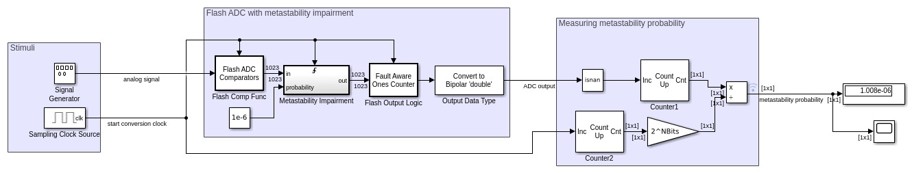
Implement Metastability Probability as an Impairment to Flash ADC

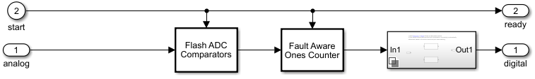
To add metastability impairment, place a triggered subsystem with a MATLAB function block after the Flash ADC Comparators subsystem. The MATLAB function block sets thermometer code signals to NaNs with a probability from a uniform random number generator. The block resets the signals on the next relevant edge which is why a triggered subsystem is used. Use this code to implement the Metastability Impairment subsystem.

%  function y = metastability(u, Probability)
%   mult = ones(size(u));
%   mult(rand(size(u)) < Probability(1)) = NaN; % metastability = NaN
%   y = u .* mult;
%  end

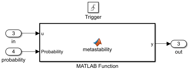
Provide the metastability probability that you want to implement through a constant block connected to the Probability port.

Implement Measuring Metastability Probability

To measure metastability impairment, count the number of NaNs encountered and divide that by the number of total comparator outputs generated during the complete simulation. A simple Simulink implementation of metastability probability measurement is:

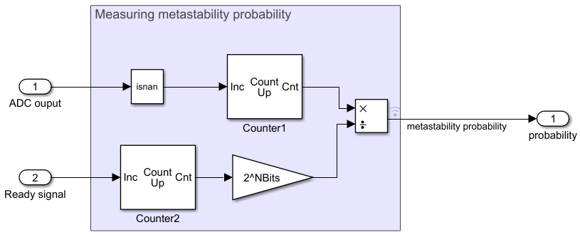
The Inports are:

ADC output- Receives the output digital code generated by the flash ADC.

Ready signal- Receives the ready signal which represents the rate at which the digital conversion is taking place. The digital code gets generated at each rising edge of the signals received by 'Ready signal' port.

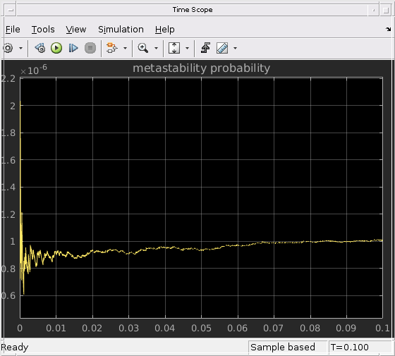
Simulation for Metastability Measurement

The model below combines the customized flash ADC with its output connected to the metastability probability measurement system. In the model, you have a 10-bit flash ADC with metastability probability of 1e-6 added. The Stimuli subsystem generates an analog signal of 100 Hz and a start conversion clock with a frequency of 100 MHz. The ADC operates at the rate defined by the start conversion clock frequency. A dashboard scope provides the behavior of the probability number over time. A display block shows the current probability being measured by the subsystem. You must run the simulation for a long enough period to see the probability number settled at the desired value, in this case 1e-6.

NBits=10;
model1='flashAdc_metastability.slx';
open_system(model1);
open_system([bdroot,'/Time Scope']);
sim(model1);

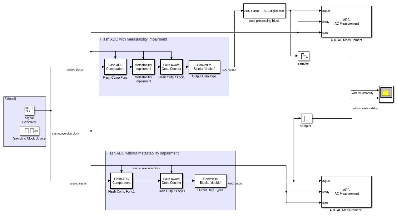
Effect of Metastability on Dynamic Performance of ADC

You can observe the effect of metastability on the dynamic performance of ADCs. The model shows two setup of flash ADC systems: one with metastability and the other without. A postprocessing block that takes in the impaired digital output and converts the NaNs to zeros. This is because the digital output with NaNs cannot be recognized by a spectrum analyzer as valid signal for spectral analysis. Attach an ADC AC measurement block to observe various performance metrics like SNR, ENOB, noise floor and so on. The simulation results show the AC analysis causes a significant drop in performance for ADC with metastability, as shown by the lower ENOB and higher noise floor.

model2='flashAdc_metastability_Effect.slx';
open_system(model2);
%To perform simulation, type the following on MATLAB prompt
%sim(model2);