Digital Timing Using Solutions to Ordinary Differential Equations

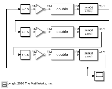
This example shows how to model a three stage ring oscillator using models defined by ordinary differential equations (ODE).

This example is the third of three examples that use a three stage ring oscillator model to explore the range of options for simulating the analog applications of digital circuits. The delays in each stage determine the ring oscillator's output frequency, making the accurate modeling of these delays essential to the simulation of the circuit.

The first two examples in the sequence, Logic Timing Simulation and Digital Timing Using Fixed Step Sampling, contain background information about this example. Read them first, in sequence, if you have not already done so.

This model uses blocks defined by ODEs, and depends on the services of an ODE solver. For each stage, the zero crossing detection capabilities of a Compare To Constant block are used to produce a saturated input to the inverter. The inverter output is converted from Boolean to double to drive a Transfer Function block. The Transfer Function block defines the shape of the inverter output transitions.

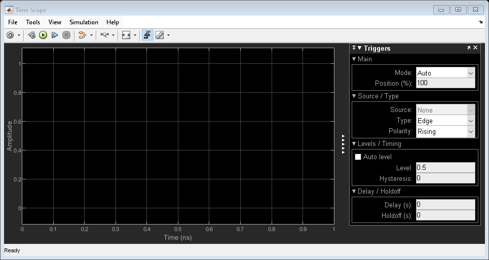
Load the ODE-based model and update the model to display sample times.

open_system('OdeWaveform');
set_param(gcs,'SimulationCommand','update');

Continuous Time Model Using Exponential Decay

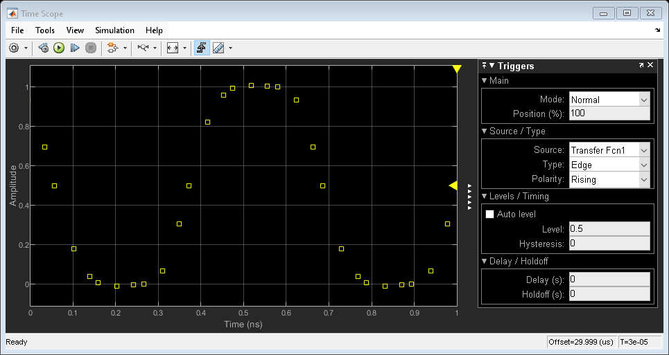
In this section, use a single pole response to evaluate the ring oscillator output when the inverter output is modeled as the response of an RC circuit.

For this section, the Transfer Function blocks are configured for a single pole response. The pole for one of the logic stages is set to a slightly different value than for the other two stages so that the model will enter the correct mode of oscillation.

The solver selection is set to auto, with a Relative Tolerance of 1e-9.

Run the ODE-based model with the single pole rise/fall response.

sim('OdeWaveform');

Continuous Time Model with Nearly Constant Slew Rate

In this section, model the response of the ring oscillator stages using a continuous time Transfer Function block with a fourth order Bessel-Thompson response to approximate a constant slew rate response.

Set the configuration for the fourth order Bessel-Thompson rise/fall response.

den = getBesselDenominator(3e9);
set_param('OdeWaveform/Transfer Fcn','Denominator',mat2str(den));
set_param('OdeWaveform/Transfer Fcn1','Denominator',mat2str(den));
den = getBesselDenominator(3.1e9);
set_param('OdeWaveform/Transfer Fcn2','Denominator',mat2str(den));

Run the modified ODE-based model. Note the slight rounding of the onset of the switching edges, similar to the waveforms produced in the Digital Timing Using Fixed Step Sampling example.

sim('OdeWaveform');

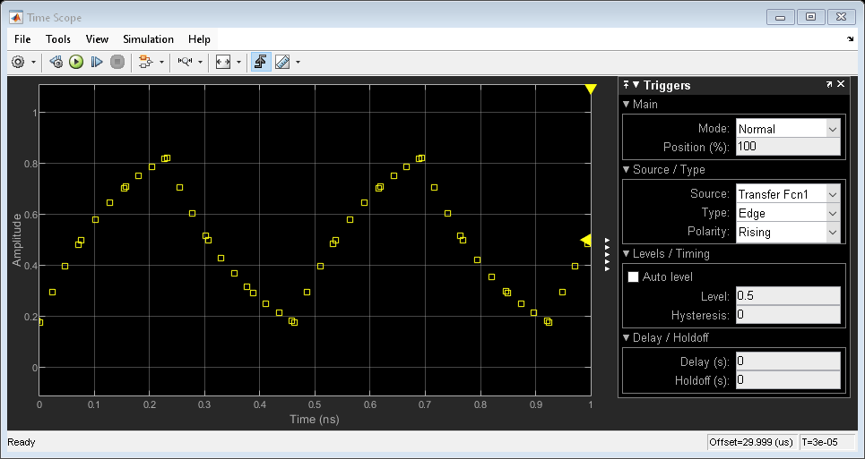
Continuous Time with Solver in Auto Mode

In this section, change the solver configuration and observe the change in results.

For circuits which are adequately described by linear, time invariant models, the combination of fixed step and variable step discrete sample times, as described in the Combined Fixed Step and Digital Timing section may be the simplest way to get reliable results. However, for circuits which must be modeled by a nonlinear or time-varying model, the ODE-based solution is the only viable option. In such cases, you should vary the maximum error tolerance, maximum step size or choice of solver in the solver configuration dialog and compare the results to the behavior you expect.

Maintain the model configuration of the previous section but change the solver's Relative Tolerance from 1e-9 to auto.

set_param('OdeWaveform','RelTol','auto');

Run the model with the auto solver setting. Observe both the change in period of oscillation and in wave shape.

sim('OdeWaveform');

Related Topics

• Logic Timing Simulation
• Digital Timing Using Fixed Step Sampling