Solve Custom MPC Quadratic Programming Problem and Generate Code
This example shows how to use the built-in active-set QP solver to implement a custom MPC algorithm that supports C code generation in MATLAB®.
Define Plant Model
The plant model is a discrete-time state-space system and it is open-loop unstable. We assume that all the plant states are measurable. Therefore, we avoid the need for designing a state estimator, which is beyond the scope of this example.
A = [1.1 2; 0 0.95];
B = [0; 0.0787];
C = [-1 1];
D = 0;
Ts = 1;
sys = ss(A,B,C,D,Ts);
x0 = [0.5;-0.5]; % initial states at [0.5 -0.5]
Design Unconstrained Linear Quadratic Regulator (LQR)
Design an unconstrained LQR with output weighting. This controller serves as the baseline to compare with the custom MPC algorithm. The LQ control law is u(k) = -K_lqr*x(k).
Qy = 1;
R = 0.01;
K_lqr = lqry(sys,Qy,R);
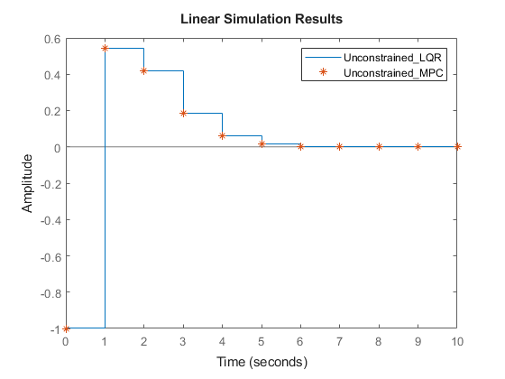
Run a simulation with initial states at [0.5 -0.5]. The closed-loop response is stable.
t_unconstrained = 0:1:10;
u_unconstrained = zeros(size(t_unconstrained));
Unconstrained_LQR = tf([-1 1])*feedback(ss(A,B,eye(2),0,Ts),K_lqr);
lsim(Unconstrained_LQR,'-',u_unconstrained,t_unconstrained,x0);
hold on

Design Custom MPC Controller with Terminal Weight
Design a custom MPC controller with the terminal weight applied at the last prediction step.
The predicted state sequences, X(k), generated by the linear model and input sequence, U(k), can be formulated as: X(k) = M*x(k) + CONV*U(k). In this example, use four prediction steps (N = 4).
M = [A;A^2;A^3;A^4];
CONV = [B zeros(2,1) zeros(2,1) zeros(2,1);...
        A*B B zeros(2,1) zeros(2,1);...
        A^2*B A*B B zeros(2,1);...
        A^3*B A^2*B A*B B];
The MPC objective function is J(k) = sum(x(k)'*Q*x(k) + u(k)'*R*u(k) + x(k+N)'*Q_bar*x(k+N)). To ensure that the MPC objective function has the same quadratic cost as the infinite horizon quadratic cost used by LQR, terminal weight Q_bar is obtained by solving the following Lyapunov equation:
Q = C'*C;
Q_bar = dlyap((A-B*K_lqr)', Q+K_lqr'*R*K_lqr);
Convert the MPC problem into a standard QP problem, which has the objective function J(k) = U(k)'*H*U(k) + 2*x(k)'*F'*U(k).
Q_hat = blkdiag(Q,Q,Q,Q_bar);
R_hat = blkdiag(R,R,R,R);
H = CONV'*Q_hat*CONV + R_hat;
F = CONV'*Q_hat*M;
When there are no constraints, the optimal predicted input sequence U(k) generated by MPC controller is -K*x, where K = inv(H)*F.
K = H\F;
In practice, only the first control move u(k) = -K_mpc*x(k) is applied to the plant (receding horizon control).
K_mpc = K(1,:);
Run a simulation with initial states at [0.5 -0.5]. The closed-loop response is stable.
Unconstrained_MPC = tf([-1 1])*feedback(ss(A,B,eye(2),0,Ts),K_mpc);
lsim(Unconstrained_MPC,'*',u_unconstrained,t_unconstrained,x0)
legend show

LQR and MPC controllers produce the same result because the control laws are the same.
K_lqr
K_mpc
K_lqr =

    4.3608   18.7401


K_mpc =

    4.3608   18.7401
LQR Control Performance Deteriorates When Applying Constraints
Restrict the controller output, u(k), to be between -1 and 1. The LQR controller generates a slow and oscillatory closed-loop response due to saturation.
x = x0;
t_constrained = 0:40;
for ct = t_constrained
    uLQR(ct+1) = -K_lqr*x;
    uLQR(ct+1) = max(-1,min(1,uLQR(ct+1)));
    x = A*x+B*uLQR(ct+1);
    yLQR(ct+1) = C*x;
end
figure
subplot(2,1,1)
plot(t_constrained,uLQR)
xlabel('time')
ylabel('u')
subplot(2,1,2)
plot(t_constrained,yLQR)
xlabel('time')
ylabel('y')
legend('Constrained LQR')

MPC Controller Solves QP Problem Online When Applying Constraints
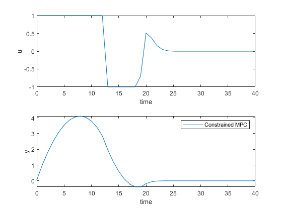
One of the major benefits of using MPC controller is that it handles input and output constraints explicitly by solving an optimization problem at each control interval.
Use the built-in KWIK QP solver, mpcActiveSetSolver, to implement the custom MPC controller designed above. The constraint matrices are defined as Ac*x>=b0.
Ac = [1 0 0 0;...
      -1 0 0 0;...
       0 1 0 0;...
       0 -1 0 0;...
       0 0 1 0;...
       0 0 -1 0;...
       0 0 0 1;...
       0 0 0 -1];
b0 = [1;1;1;1;1;1;1;1];
Because in this case the Hessian matrix H is constant, you can precalculate the inverse of its lower-triangular Cholesky decomposition, and then pass it to the mpcActiveSetSolver function, instead of passing the Hessian matrix directly. As a result, mpcActiveSetSolver can avoid performing this computation at each time step.
L = chol(H,'lower');
Linv = L\eye(size(H,1));
Run a simulation by calling mpcActiveSetSolver at each simulation step. Initially all the inequalities are inactive (cold start).
x = x0;
iA = false(size(b0));

% create options for the solver, and specify non-hessian first input
opt = mpcActiveSetOptions('IntegrityChecks',false,'UseHessianAsInput',false);
for ct = t_constrained
    [u,status,iA] = mpcActiveSetSolver(Linv,F*x,Ac,b0,[],zeros(0,1),iA,opt);
    uMPC(ct+1) = u(1);
    x = A*x+B*uMPC(ct+1);
    yMPC(ct+1) = C*x;
end
figure
subplot(2,1,1)
plot(t_constrained,uMPC)
xlabel('time')
ylabel('u')
subplot(2,1,2)
plot(t_constrained,yMPC)
xlabel('time')
ylabel('y')
legend('Constrained MPC')

The MPC controller produces a closed-loop response with faster settling time and less oscillation.
Simulate Custom MPC Using MATLAB Function Block in Simulink
mpcActiveSetSolver can be used inside a MATLAB Function block to provide simulation and code generation in the Simulink® environment.
mdl = 'mpc_activesetqp';
open_system(mdl)


The Custom MPC Controller block is a MATLAB Function block. To examine the MATLAB code, double-click the block. Because Linv, F, Ac, b0 matrices, and opt structure are constant, they are passed into the MATLAB Function block as parameters.
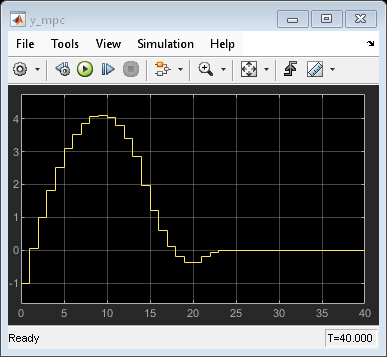
Run a simulation in Simulink. The closed-responses of LQR and MPC controllers are identical to their counterparts in the MATLAB simulation.
open_system([mdl '/u_lqr'])
open_system([mdl '/y_lqr'])
open_system([mdl '/u_mpc'])
open_system([mdl '/y_mpc'])
sim(mdl)


Code Generation in MATLAB
mpcActiveSetSolver supports C code generation with MATLAB Coder™. Assume you have a function, mycode, that is, compatible with the code generation standard.
function [x,iter,iA1,lam] = mycode()
%#codegen
n = 5;
m = 10;
q = 2;
H = diag(10*rand(n,1));
f = randn(n,1);
A = randn(m,n);
b = randn(m,1);
Aeq = randn(q,n);
beq = randn(q,1);
Linv = chol(H,'lower')\eye(n);
iA = false(m,1);
opt = mpcActiveSetOptions('IntegrityChecks',false,'UseHessianAsInput',false);
[x,iter,iA1,lam] = mpcActiveSetSolver(Linv,f,A,b,Aeq,beq,iA,opt);
You can use following command to generate C code with MATLAB Coder:
fun = 'mycode';
Cfg = coder.config('mex'); % or 'lib', 'dll', etc.
codegen('-config',Cfg,fun,'-o',fun);
Acknowledgment
This example is inspired by Professor Mark Cannon's lecture notes for the Model Predictive Control class at University of Oxford. The plant model is the same one used in Example 2.1 in the "Prediction and optimization" section.
bdclose(mdl)
See Also
Functions
mpcmove|mpcActiveSetSolver|mpcInteriorPointSolver|setCustomSolver|quadprog(Optimization Toolbox)