Get Started with Medical Volume Viewer

Since R2026a

The Medical Volume Viewer app enables you to visualize 3-D medical image volumes, including label data and multimodal overlays. You can explore volumes in 3-D or as 2-D slice planes, apply and customize transparency and colormaps, and view multimodal images, such as CT and PET, together as an overlay. You can publish 2-D and 3-D snapshots and animations, and export display settings to apply outside the app.

This tutorial provides an overview of the capabilities of the Medical Volume Viewer.

Download Data

This example explores chest CT data from a subset of the Medical Segmentation Decathlon data set [1]. Download the MedicalVolumeNIfTIData.zip file from the MathWorks® website, then unzip the file. The size of the subset of data is approximately 76 MB. After you download the data, the dataFolder folder contains the downloaded and unzipped data.

zipFile = matlab.internal.examples.downloadSupportFile("medical","MedicalVolumeNIfTIData.zip");
filepath = fileparts(zipFile);
dataFolder = fullfile(filepath,"MedicalVolumeNIfTIData");

if ~exist(dataFolder)
    unzip(zipFile,filepath)
end

Read one of the CT volumes and its tumor label mask into the workspace as medicalVolume objects.

ctVol = medicalVolume(fullfile(dataFolder,"lung_027.nii.gz"));
labelVol = medicalVolume(fullfile(dataFolder,"LabelData","lung_027.nii.gz"));

Open Medical Volume Viewer App

Open the Medical Volume Viewer app from the Apps tab on the MATLAB® Toolstrip, under Image Processing and Computer Vision. You can also load the app by using the medicalVolumeViewer command.

At any time, you can start a new app session by selecting New Session in the app toolstrip. When you create a new session, this option deletes all the data currently in the app.

Import Data

You have several options for importing data. Choose the option that is convenient for you while including any metadata available from the original data source. For example, import a DICOM volume from the file, or from a medicalVolume object created from the file, rather than a 3-D numeric array containing only the voxel data. If you specify a file with limited metadata, such as a TIFF file, or a 3-D numeric array of voxel values without metadata, the app assumes default spatial referencing with voxel spacing of 1-by-1-by-1 millimeters, with the first voxel located at (1, 1, 1). The app also hides anatomical plane and direction labels.

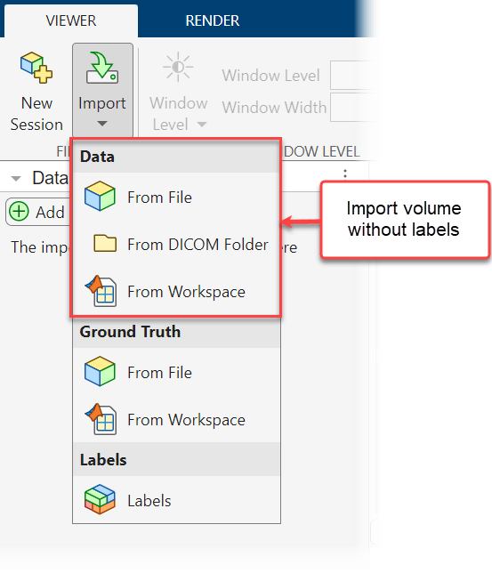
Import Volumes Without Labels

To import unlabeled volumes into the app interactively, select Import from the Viewer tab of the app toolstrip and, under Data, select one of these options:

• From File — Import NIfTI, NRRD, TIFF, DICOM, or MAT files. Each DICOM file must contain a complete volume. Each MAT file must contain a medicalVolume object or a 3-D numeric array.

• From DICOM Folder — Import a folder of DICOM files that define one multi-file volume.

• From Workspace — Import a medicalVolume object or a 3-D numeric array of voxel data.

Alternatively, to import an unlabeled volume programmatically, use the syntax medicalVolumeViewer(volume), where volume is a filename, DICOM folder name, medicalVolume object, or 3-D numeric array.

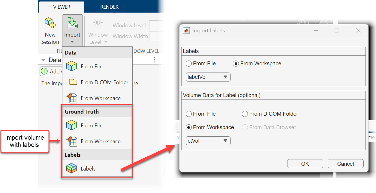
Import Volumes with Labels

To import a labeled volume into the app interactively, select Import from the Viewer tab of the app toolstrip and select one of these options.

• Under Ground Truth, select From File — Import a MAT file that contains a groundTruthMedical object specifying the label definitions and paths to the volume and label data.

• Under Ground Truth, select From Workspace — Import a groundTruthMedical object from the workspace.

• Select Labels — Import labels and volume data using an interactive dialog box. In the Import Labels dialog box, select whether to import the label data from a file or from a workspace variable. Label data files can be in the NIfTI, DICOM, NRRD, or MAT format. A DICOM file must contain a complete volume. A MAT file must contain a medicalVolume object or a 3-D numeric array. If you choose to import labels from the workspace, you can pick a medicalVolume object or 3-D numeric array from the drop-down in the Labels section. The dialog box also contains a Volume Data for Label section, in which you can optionally specify a volume to associate with the labels. If you specify a file or workspace variable, the app imports the volume with the labels. If you specify a volume already in the Data Browser, the app imports the labels and associates them with the existing copy of the volume.

For this example, use the Labels option to import the CT volume and labels from the workspace. In the Import Labels dialog box, select From Workspace in both the Labels and Volume Data for Label sections, and select labelVol and ctVol from their respective drop-down lists.

Alternatively, to import a labeled volume programmatically, use the syntax medicalVolumeViewer(volume,labels) or medicalVolumeViewer(gTruth), where volume specifies a volume, labels specifies label data, and gTruth specifies a groundTruthMedical object in the workspace or a file that contains a groundTruthMedical object.

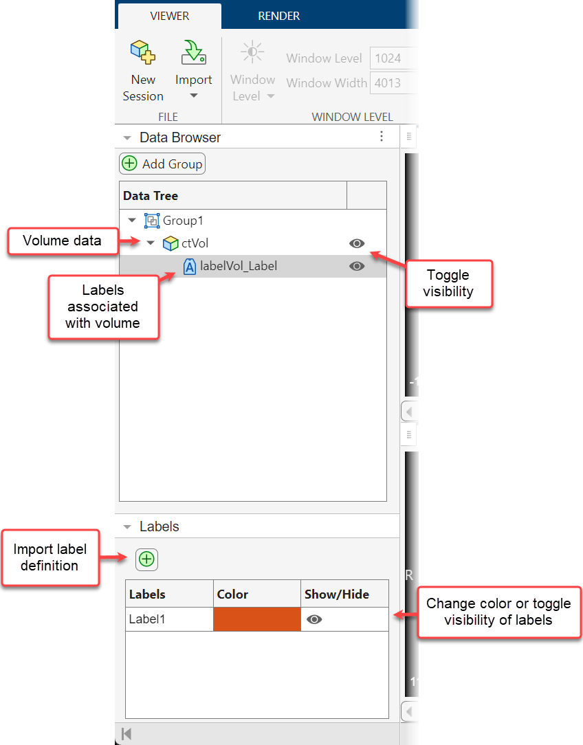
Organize Volumes and Labels

The Data Browser enables you to view and organize the volumes and labels loaded in an app session. The browser indicates volumes using the volume icon. All labels associated with a volume are in a collapsible list and are indicated using the label icon . To toggle the visibility of a volume or label, click the eye icon next to the filename. If you make multiple volumes visible, the app displays them as an overlay. You can delete a volume or label image from the app by right-clicking the name in the browser and selecting Delete Entry. You can categorize related volumes, such as all scans per patient or time point, using groups. By default, the app adds all volumes to Group 1. To create a new group, select Add Group. Drag and drop filenames to move volumes between groups. You can rename a group by double-clicking the group name and typing a new name. The appearance of the app depends on whether a volume or label is selected in the browser. For example, selecting a label image makes the Labels pane and the Label Opacity slider visible, and selecting a volume makes the Window Level and Rendering Editor buttons visible.

The Labels pane displays the name and color of each label present in the visible label files. By default, the app uses standardized display colors and numbered label names starting with Label1. If you have a label definitions file for your label data with custom names and colors, which you can export from the Medical Image Labeler app, you can import it by selecting the plus icon. You can change the display color of individual labels by double-clicking the Color column for that label and selecting a new color in the dialog box. You can toggle the visibility of individual labels by clicking the eye icon in the corresponding row of the Show/Hide column.

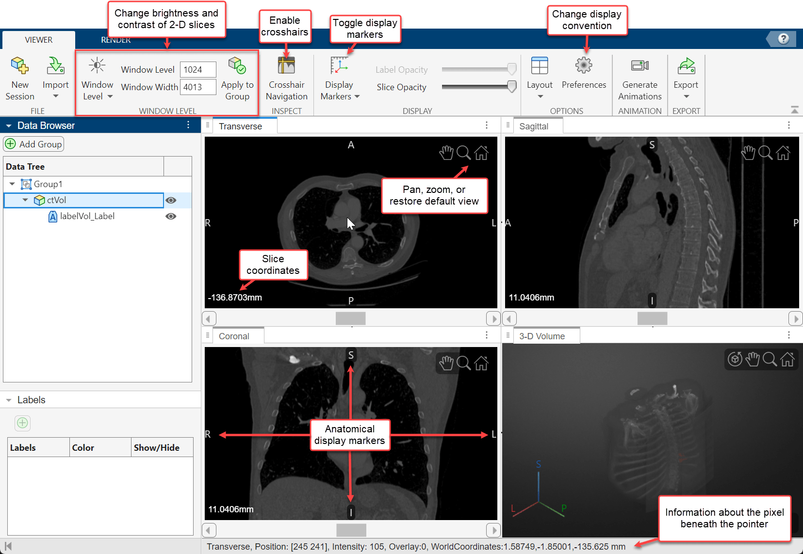
Explore Volume Data

The app displays volumes as 2-D slice planes and a 3-D volume in a four-pane view. The 2-D slices are displayed in the Transverse, Sagittal, and Coronal planes. If your volume has incomplete or oblique spatial metadata, the app displays the volume without anatomical labels.

View 2-D Slices

To explore the volume, zoom in on a slice pane using the scroll wheel or the zoom controls in the top-right corner of the slice. Navigate between slices by using the scroll bar in each of the 2-D slice panes. The app also displays anatomical display markers indicating the anterior (A), posterior (P), left (L), right (R), superior (S), and inferior (I) directions. Labels in the bottom-left corner of each slice pane indicate the slice position in world coordinates, the current slice number, and the total number of slices in that dimension. When you display multiple volumes or labels as an overlay, the app hides the slice numbers and shows only the position values. The bottom of the app window displays information about the pixel beneath the pointer, including its coordinates and intensity. Note that, if you import a volume with limited spatial metadata, the app hides the anatomical display markers.

You can also navigate between slices in the three planes using crosshair navigation. To turn on the crosshair indicators, in the Viewer tab of the app toolstrip, select Crosshair Navigation. The indicators in each 2-D view show the relative positions of the current slices in the other 2-D views. To navigate slices, drag the crosshairs to a new position. The other slice views update automatically. To hide the crosshairs, in the app toolstrip, clear Crosshair Navigation.

By default, the app displays volumes using the Radiological display convention, with the left side of the patient on the right side of the image. To display the left side of the patient on the left side of the image, on the app toolstrip, click Preferences, and in the dialog box that opens, change Convention to Neurological.

To change the brightness or contrast of the display, adjust the display window. To update the display window, you can directly edit the values in the Window Level and Window Width boxes in the app toolstrip. Alternatively, adjust the window using the Window Level tool. First, select the window level button in the app toolstrip. Then, drag up and down in a 2-D view pane to increase and decrease the brightness, respectively, or left and right to increase and decrease the contrast for all of the 2-D views. The Window Level and Window Width values in the toolstrip automatically update when you release the mouse button. Clear the window level button to deactivate the tool. To apply window level changes to all volumes within the same group in the Data Browser, select Apply to Group. To reset the brightness and contrast, click Window Level and select Reset.

View 3-D Volume

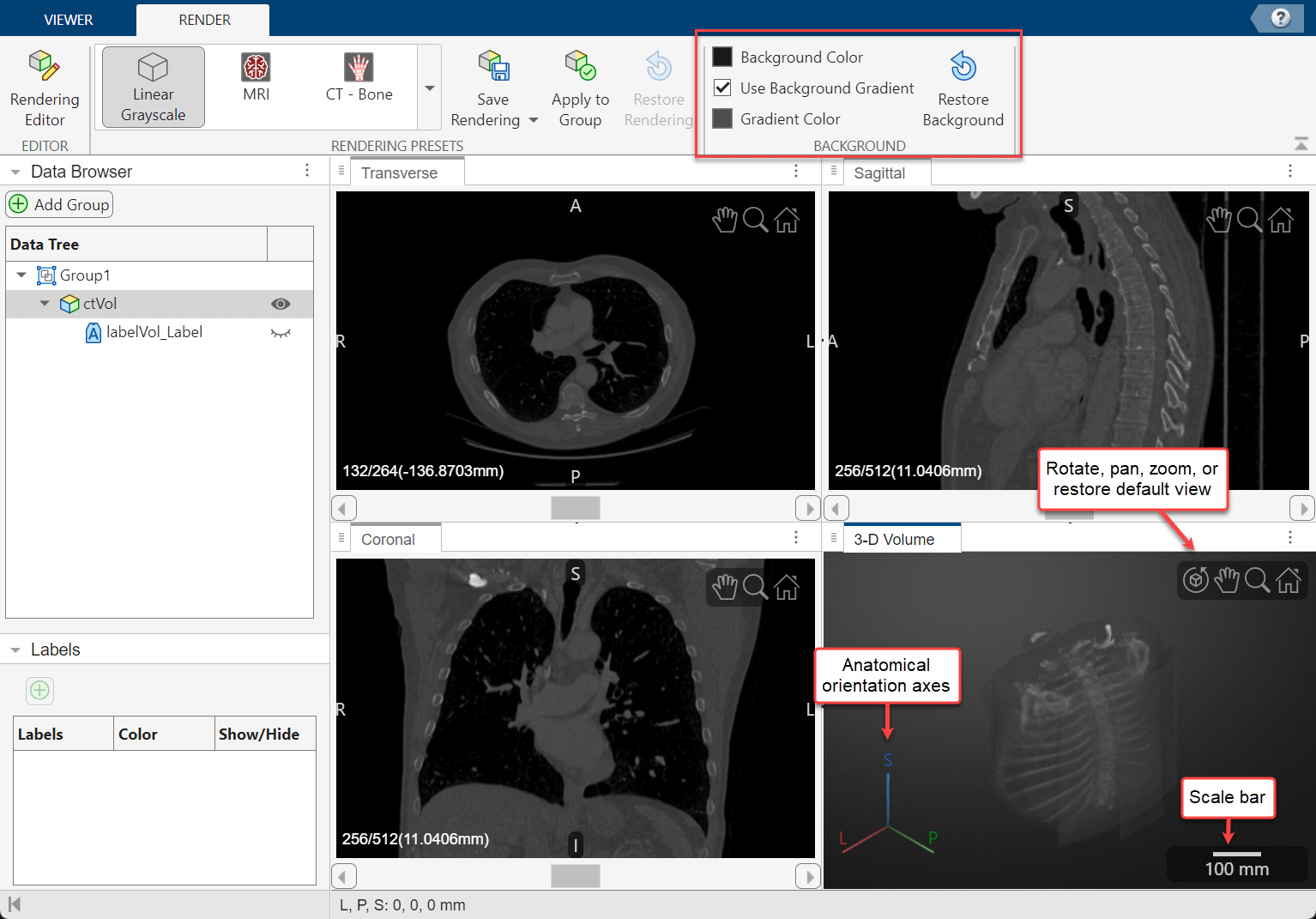
In the 3-D Volume pane, you can zoom using the scroll wheel or rotate the volume about its center by dragging it. The orientation axes in the bottom-left corner indicate the spatial orientation of the volume. The scale bar in the bottom-right corner provides an indication of the volume size. To toggle the visibility of the orientation axes and scale bar, select Display Markers in the app toolstrip and select or clear the 3-D Orientation Axes and Scale Bars options under 3-D Volume, respectively.

You can change the background color or apply a background gradient to the 3-D Volume pane from the Render tab of the app toolstrip. To change the background color, select Background Color and select a color. Clear or select the Use Background Gradient box to toggle the visibility of the background gradient. To change the gradient color, select Gradient Color and select a color.

Refine Display

This part of the example describes how to modify the appearance of the data. Using the app, you can:

• Apply preset styles that apply transparency and colormaps that work well for medical data.

• Change the rendering technique for the 3-D volume.

• Modify the preset rendering styles by interactively modifying the intensity-opacity curve and color bar scale.

• Control the visibility and color of label data.

Apply Rendering Preset

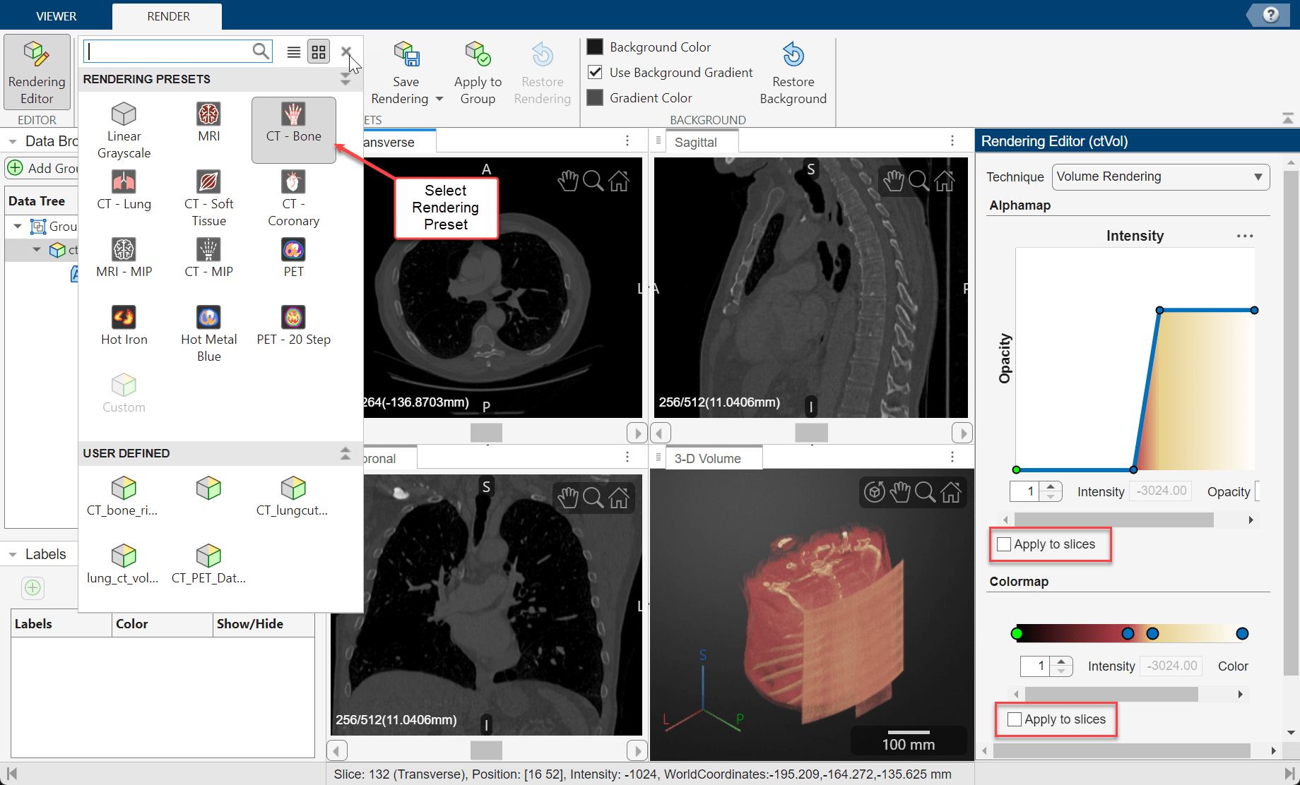
The app provides several built-in rendering presets that apply alphamaps and colormaps that work well with medical images, such as CT-Bone, MRI, and PET. To apply a preset to the currently selected volume, in the Render tab of the app toolstrip, select an option from the Rendering Presets gallery.

By default, the preset applies only to the 3-D Volume display pane. You can optionally apply the preset to the 2-D slices by opening the Rendering Editor from the app toolstrip and, under Alphamap and Colormap, selecting Apply to slices. Otherwise, the slices display with a grayscale colormap and a constant transparency that you can modify by using the Slice Opacity slider on the Viewer tab of the app toolstrip.

Choose Rendering Technique

You can adjust the appearance of the 3-D Volume pane by changing the rendering technique in the Rendering Editor. To open the editor, in the Render tab of the app toolstrip, click Rendering Editor. You can choose one of these options.

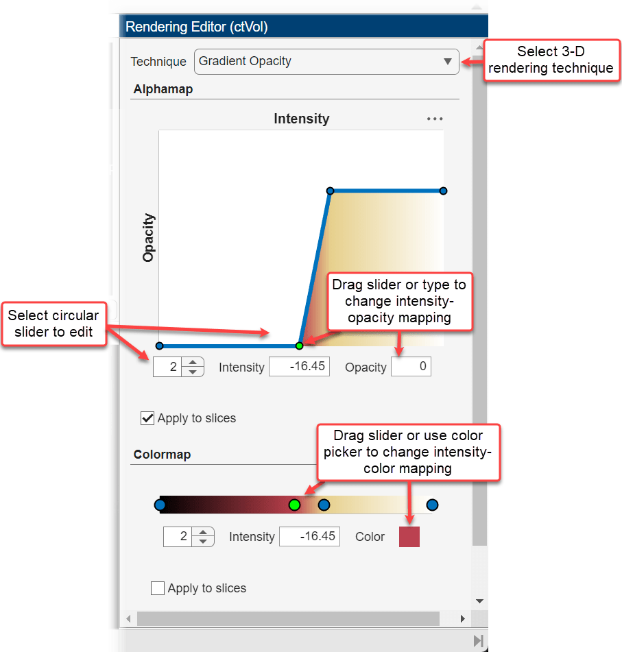
• Volume Rendering — View the volume based on the color and transparency for each voxel, as specified by the colormap and alphamap.

• Cinematic Rendering — View the volume based on the specified color and transparency for each voxel, with iterative postprocessing that produces photorealistic shadows and lighting. This technique is useful for displaying opaque volumes, but can take longer to render.

• Minimum Intensity Projection — View the voxel with the smallest intensity value for each ray projected through the data.

• Maximum Intensity Projection — View the voxel with the largest intensity value for each ray projected through the data. This technique can be useful for revealing the highest-intensity structure within a volume.

• Gradient Opacity — View the volume based on the specified color and transparency, with an additional transparency applied if the voxel is similar in intensity to the previous voxel along the ray projected through the data. When you render a volume with uniform intensity using this technique, the interior appears more transparent than when displayed using Volume Rendering, enabling better visualization of intensity gradients within the volume.

• Isosurface — View the volume as an isosurface. The default isovalue is 0.5.

• Slice Planes — View the volume as three orthogonal slice planes. You can change the position of each slice by pausing on a slice plane until it highlights, and then dragging it.

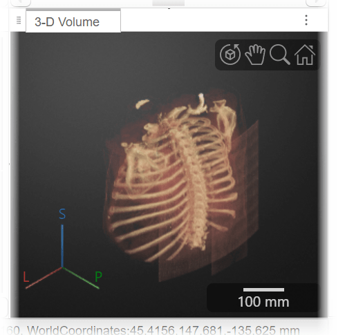
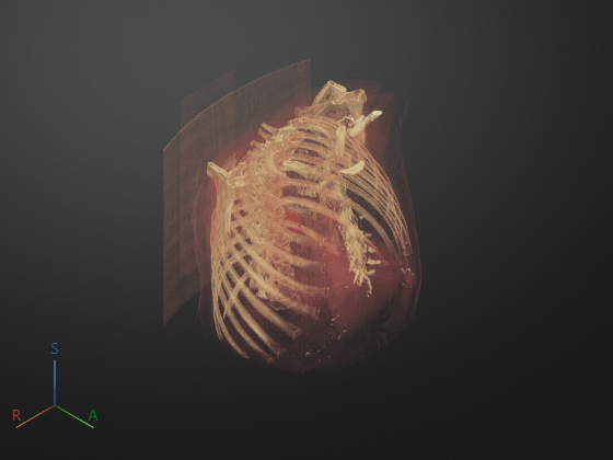
For this example, select Gradient Opacity. Changing the rendering technique improves the visibility of the internal bone structures.

Customize Alphamap and Colormap

You can refine the preset alphamap and colormap for your data by modifying the intensity-opacity curve and colormap in the Rendering Editor.

In the Alphamap section, the intensity-opacity curve maps voxel intensity to opacity for points defined by circular sliders. For example, the alphamap for the Linear Grayscale preset has two circular sliders that map the minimum intensity to an opacity of 0 and the maximum intensity to an opacity of 1. The app interpolates opacity values for intensities between the circular sliders. You can add sliders by clicking the line plot. You can change the intensity associated with a slider by dragging it left and right on the plot, or by selecting it and specifying a new value for Intensity. You can change the opacity associated with a slider by dragging it up and down on the plot, or by selecting it and specifying a new value for Opacity.

In the Colormap section, the color bar scale maps voxel intensity to colors for points defined by circular sliders. For example, the Linear Grayscale preset maps the minimum intensity to black and the maximum intensity to white, interpolating colors between the sliders. You can refine the colormap by adding or editing sliders. Click the color bar to add a slider. Change the intensity of a slider by dragging it horizontally, or selecting it and specifying a new value for Intensity. You can change the mapping of a slider by clicking the Color box, selecting a new color from the Color dialog box, then clicking OK. The color under the intensity-opacity plot updates to reflect the updated colormap.

To save your customized settings, in the Render tab of the app toolstrip, click Save Rendering . The app adds an icon for your custom preset to the gallery in the Rendering Presets section of the app toolstrip, under User Defined. You can apply the same preset or custom rendering settings to all volumes in a Data Browser group by clicking Apply To Group in the app toolstrip. To discard your customizations, select Restore Rendering.

Export Snapshot Images

You can export snapshot images of 2-D and 3-D views to use outside the app. In the Viewer tab of the app toolstrip, select Export > Slices. In the Export Slices dialog box, select the views you want to export, choose whether to save images as PNG images or a PDF, and click Export. In the next dialog box, specify the location where you want to save the images. If you export images, you must specify a folder, as each snapshot is saved as a separate PNG file. If you export a PDF, you must specify a filename, as the slices are published in a single document.

Export Animations

You can generate 2-D animations that scroll through transverse, sagittal, or coronal slices, or 3-D animations of the volume rotating about a specified axis. To open the animation generator tool, in the Viewer tab of the app toolstrip, click Generate Animations.

Create 2-D Animation

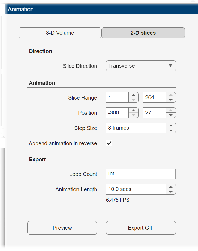
To export a 2-D animation, in the Animation editor, select 2-D slices. In the Direction section, specify the Slice Direction along which you want to view slices. In the Animation section, specify which slices to include in the animation based on slice number or coordinates using the Slice Range or Position option, respectively, and adjust the Step Size. Select Append animation in reverse to make the animation scroll forward and then backward through the slices, rather than forward only. In the Export section, specify the Loop Count and Animation Length. The loop count is the number of times to repeat the animation, equivalent to specifying the LoopCount name-value argument of imwrite. Specify the loop count as a positive integer, for a fixed number of loops, or as Inf to create a continuously looping animation. Specify the animation length in seconds. The editor displays the speed of the animation in frames per second based on your specified slice range and animation length.

For this example, specify these values to create an animation that captures every eighth slice along the transverse direction.

• Specify the Slice Direction as Transverse.

• Keep the default values for the minimum and maximum of Slice Range as 1 and 264, respectively.

• Keep the default values for the minimum and maximum of Position as -300 and 27, respectively.

• Specify the step size as 8 frames.

• Select Append animation in reverse so each loop animates forward and then in reverse through the slice range.

• Keep the default value for Loop Count as Inf to create an animation that loops infinitely.

• Keep the default value for Animation Length as 10.0 secs.

Click Preview to preview one loop of the animation with the specified Direction and Animation settings. The preview does not reflect the loop count or animation length of the exported GIF. The preview plays in the slice view of the selected slice direction. If you are satisfied with the preview, click Export GIF, and, in the dialog box, select the location to save the animation GIF file. You can open and view the GIF file from the saved location and share the animation outside of MATLAB.

Create 3-D Animation

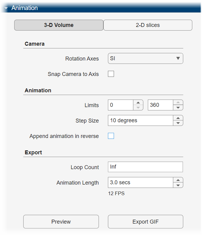
To export a 3-D animation, in the Animation pane, select 3-D Volume. Under Camera, specify the Rotation Axes, which indicates the axis to rotate around, as SI (superior-inferior), LR (left-right), AP (anterior-posterior), or the current up vector in the 3-D Volume pane. When you specify the rotation axis as SI, LR, or AP, by default the app generates the image using the current camera position in the 3-D Volume pane, including any rotations you have applied. In this case, if you want to generate an animation that views the plane orthogonal to the rotation axis, select Snap Camera to Axis. When you specify the rotation axis as Current Up Vector, the Snap Camera to Axis option is unavailable. In the Animation section, use Limits to specify the minimum and maximum angles around the axis, in degrees, between which to rotate the volume. Specify the Step Size in degrees.

For this example, specify these values to create an animation of the volume rotating about the superior-inferior axis, with frames acquired every ten degrees of rotation.

• Specify the Rotation Axes as SI.

• Keep the default values for the minimum and maximum of Limits as 0 and 360, respectively.

• Specify the step size as 8 frames.

• Clear Append animation in reverse so the animation rotates only one direction around the axis.

• Keep the default value for Loop Count as Inf to create an animation that loops infinitely.

• Keep the default value for Animation Length as 3.0 secs.

Click Preview to preview one loop of the animation with the specified Camera and Animation settings. The preview does not reflect the loop count or animation length of the exported GIF. The preview plays in the 3-D Volume pane. If you are satisfied with the preview, click Export GIF, and, in the dialog box, select the location to save the animation GIF file. You can open and view the GIF file from the saved location and share the animation outside of MATLAB.

Export Rendering Settings

After working in Medical Volume Viewer to achieve the best view of your data, you can save your rendering settings and camera configuration to the workspace. You can apply the saved settings to recreate the view you achieved in Medical Volume Viewer by using them to set properties of the objects created by the viewer3d and volshow functions.

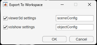
To save rendering and camera configuration settings, in the Viewer tab of the app toolstrip, click Export and, under Viewer3d Settings, select To Workspace. Medical Volume Viewer creates separate structures for the settings of objects created by viewer3d and volshow. You can choose which structures to create, and either specify their names or accept the default names sceneConfig and objectConfig, respectively. When you are ready to export, click OK.

Apply Rendering Settings Outside App

Programmatically display the volume, applying the rendering and camera settings outside the app. The new display has the same colormap, alphamap, rendering style, background color and gradient, and camera position as the 3-D Volume pane had when you exported the settings.

load("ChestCTRenderingSettings.mat")

% Create volume display

viewer = viewer3d;

Volume = volshow(ctVol,Parent=viewer, ...
DisplayRangeMode="data-range", ...
OverlayData=labelVol.Voxels);

% Apply objectConfig settings by setting Volume object properties

fields = fieldnames(objectConfig);

for i = 1:numel(fields)
    Volume.(fields{i}) = objectConfig.(fields{i});

end

% Apply sceneConfig settings by setting Viewer object properties

fields = fieldnames(sceneConfig);
for i = 1:numel(fields)

viewer.(fields{i}) = sceneConfig.(fields{i});
end

References

[1] Medical Segmentation Decathlon. "Lung." Tasks. Accessed May 10, 2018. http://medicaldecathlon.com. The Lung data set is provided by the Medical Segmentation Decathlon under the CC-BY-SA 4.0 license. All warranties and representations are disclaimed. See the license for details. This example uses a subset of the original data set consisting of two CT volumes.