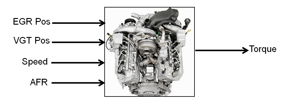
Design of Experiments for Multi-Injection Diesel Engine Calibration
Benefits of Design of Experiment
You use design of experiment to efficiently collect engine data. Testing time (on a dyno cell, or as in this case, using high-fidelity simulation) is expensive, and the savings in time and money can be considerable when a careful experimental design takes only the most useful data. Dramatically reducing test time is increasingly important as the number of controllable variables in more complex engines is growing. With increasing engine complexity, the test time increases exponentially.
Air-System Survey Testing
The first stage to solve this calibration problem is to determine the boundaries of the feasible air-system settings. To do this, create an experimental design and collect data to determine air-system setting boundaries that allow positive brake torque production in a feasible AFR range.
These simplifications were used to conduct the initial study:
Pilot injection is inactive.
Main timing is fixed.
Nominal fuel pressure vs RPM.
Main fuel mass is moved to match the AFR target.
The design process follows these steps:
Set up variable information for the experiment, to define the ranges and names of the variables in the design space.
Choose an initial model.
Create a base design that contains the correct constraints.
Create child designs using varying numbers of points and/or methods of construction.
Choose the design to run based on the statistics and how many points you can afford to run.
Create Designs and Collect Data
You can use a space-filling design to maximize coverage of the factors' ranges as quickly as possible, to understand the operating envelope.
To create a design, you need to first specify the model inputs. Open the example file to see how to define your test plan.
In MATLAB®, on the Apps tab, in the Automotive group, click MBC Model Fitting.
Select File > Open Project and browse to the example file
CI_MultiInject_AirSurvey.mat, found inmatlab\toolbox\mbc\mbctraining.The Model Browser displays the top project mode in the All Models tree,
CI_Multiinject_AirSurvey.To see how to define your test plan, click Design Experiment. In the new test plan dialog box, observe the inputs pane, where you can change the number of model inputs and specify the input symbols, signals and ranges. This example project already has inputs defined, so click Cancel.
Click the first test plan node in the All Models tree,
AirSurveyDoE. The test plan view appears.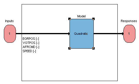
Observe the inputs listed on the test plan diagram. Double-click the Inputs block to view the ranges and names (symbols) for variables in the Input Factor Set Up dialog box.
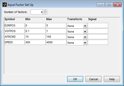
Close the dialog box.
After setting up inputs, you can create designs. In the Common Tasks pane, click Design experiment.
The Design Editor opens. Here, you can see how these designs are built:
The final Air Survey design is a ~280 point Sobol Sequence design to span the engine operating space. The Sobol Sequence algorithm generated the space-filling design points. The final design is called
AirSurveyMergedDoEbecause it contains two merged designs, one with a constraint and one unconstrained:A 232-point design for overall engine operating range called
AirSurveySpaceFillA 50-point design low speed/load for an idle region called
AirSurveyIdle
Select the
AirSurveySpaceFilldesign in the Designs tree, and select View > Current View > 2D Design Projection.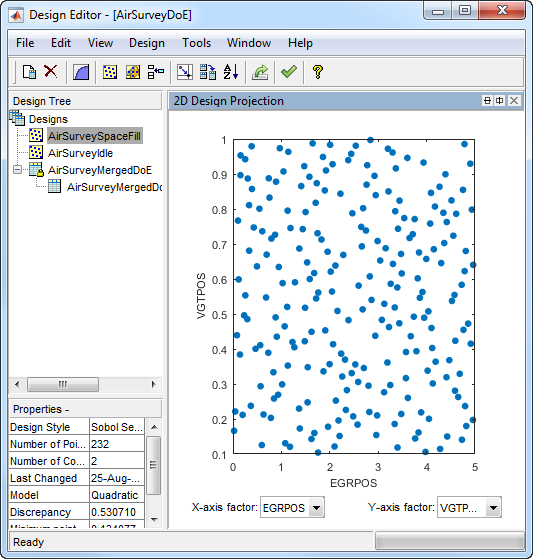
Select Edit > Constraints to see how the constraints are set up.
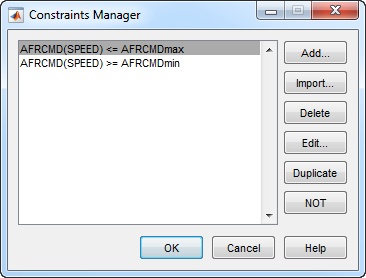
In the Constraints Manager dialog box, select a constraint and click Edit. Observe that you can define areas to exclude by dragging points or typing in the edit boxes.
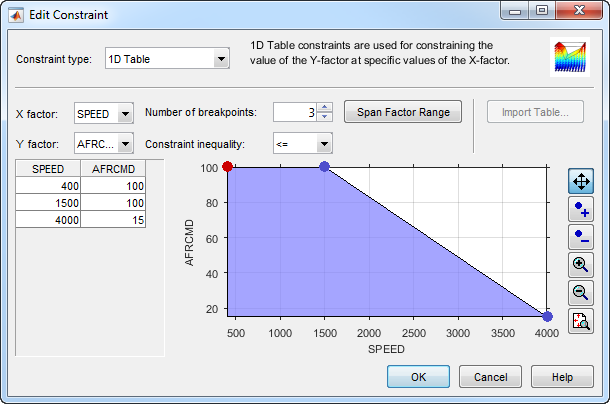
Click Cancel to close the Edit Constraint dialog box and leave the constraint unchanged. Close the Constraints Manager dialog box.
Observe the
Propertiesof the selectedAirSurveySpaceFilldesign under the tree, listing 2 constraints, 232 points, and aDesign StyleofSobol Sequence.You can see how to construct a design like this by selecting Design > Space Filling > Design Browser, or click the space-filling design toolbar button.
A dialog box asks what you want to do with the existing design points. Click OK to replace the points with a new design.
In the Space-Filling Design Browser, click Generate several times to try different space-filling points. You can specify the Number of points, and view previews of design points. Observe the default design type is
Sobol Sequence.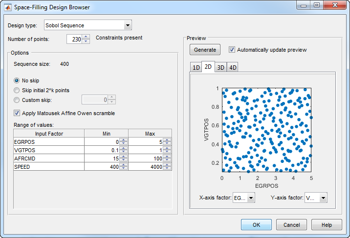
Click Cancel to close the Space-Filling Design Browser and leave the design unchanged.
Click the
AirSurveyIdledesign to observe it is also aSobol Sequencedesign, containing 50 points and no constraints.Click the
AirSurveyMergedDoEdesign to observe it is of typeCustom, and contains 282 points and 2 constraints. This design is formed by merging the previous 2 designs. You can find Merge Designs in the File menu.Click
AirSurveyMergedDoE_RoundedSorted, the child design ofAirSurveyMergedDoE. This design contains the same points but rounded and sorted, using Edit > Sort Points and Edit > Round Factor. This is the final design used to collect data.Close the Design Editor.
The final air survey design was used to collect data from the GT-Power model with the
Simulink® and Simscape™ test harness. The example Model Browser project file
CI_MultiInject_AirSurvey.mat contains this data, imported to the Model
Browser after the air survey. You can also view the data in spreadsheet form in the file
CI_AirSurvey_Data.xlsx in the mbctraining folder.
Fit a Boundary Model to Air Survey Data
You need to fit a boundary model to the data collected at the air survey design points. The
test data from the air survey was used to create a boundary model of the engine operating range.
The example Model Browser project file CI_MultiInject_AirSurvey.mat contains
this boundary model.
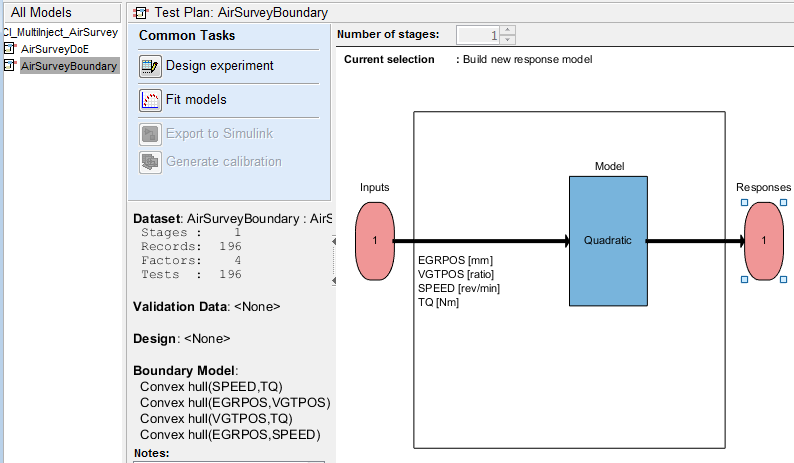
In the Model Browser, click the second test plan node in the All Models tree,
AirSurveyBoundary.Compare with the
AirSurveyDoEtest plan view. For the boundary modeling test plan,Observe an imported data set listed under the Common Tasks pane. The second test plan has imported the air survey data in order to fit a boundary model to the data.
Observe the
Inputsare different in the test plan diagram. Instead of theAFRCMDinput in the DoE test plan, there is aSPEEDinput for boundary modeling.AFRCMDwas used to constrain the design points to collect the air survey data. To model the boundary before creating the final design, you now need theSPEEDinput instead.
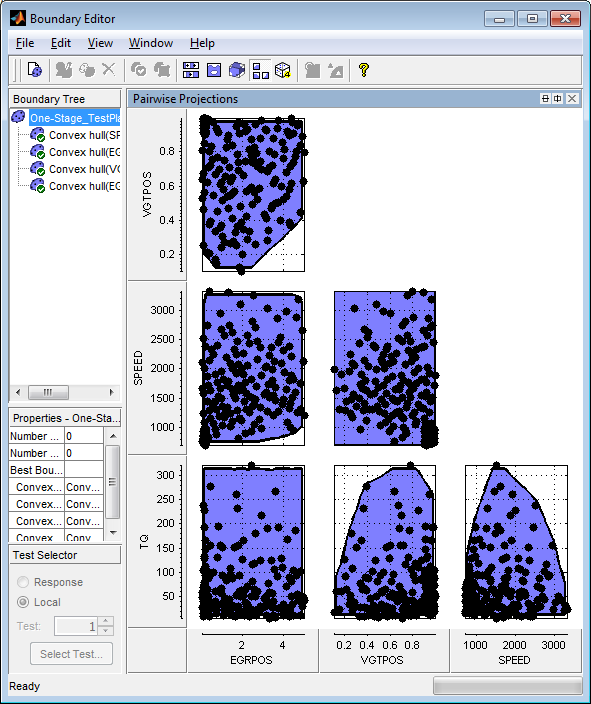
In the Model Browser, select TestPlan > Edit Boundary to open the Boundary Editor.
Examine the boundary model by selecting View > Current View > Pairwise Projections. The plots show the shape across the inputs.
Use the Air Survey and Boundary Model to Create the Final Design
The initial air survey design and test data provide information about the engine operating envelope, where the feasible AFR range can produce positive brake torque. The resulting data lets you create a boundary model. You can use the boundary model to create the final design avoiding infeasible points, and in later steps to guide modeling and constrain optimizations.
Using the boundary model as a constraint, you can generate the final design to collect detailed data about fuel injection effects within those boundaries. You can then use this data to create response models for all the responses you need in order to create an optimal calibration for this engine.
The final Point-by-Point Multi-Injection design (around 7000 points) was generated using a MATLAB script together with the Air Survey boundary model.
Open the example files
CI_PointbyPointDoE.mandcreateCIPointbyPointDoEs.min thembctrainingfolder to see the script commands that build the final design.The script keeps only points that lie within the boundary model, and continues generating design points until it reaches the desired number of points. The Sobol space-filling design type keeps filling in spaces for good coverage of the design space.
After generating design points for each test, the script creates a Model Browser project with a point-by-point test plan, and attaches the point-by-point designs to the test plan.
Open the project
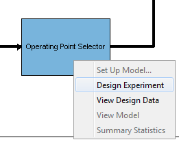
CI_MultiInject_PointbyPoint.matto view the project created by the script.Select the second test plan node in the tree, and then click the Test Plan tab. In the test plan diagram, right-click the Operating Point Selector block, and select Design Experiment to view the designs created by the script.
In the Design Editor, select Mode Points in the Design tree, and view the 2D Design Projection.
In the Design tree, select Actual Design. Observe that the boundary model constraint removed points in the corners, so that the actual design points collect data only in the feasible region determined by the initial air survey.
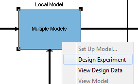
Return to the Model Browser test plan, right-click the Local Model block, and select Design Experiment.
Click test numbers to view the local design points at each operating point. At each test, the values of
SPEEDandTQare fixed and the space-filling design selects points across the space of the local inputs.
Multi-Injection Testing
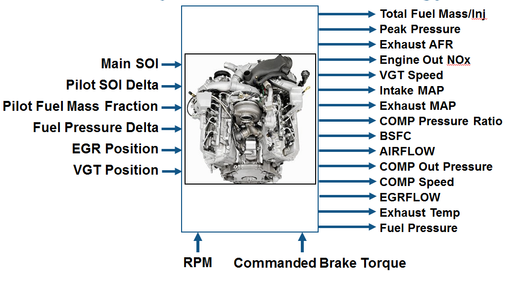
The final design was used to collect data for the following inputs and responses.
The toolbox provides the data files for you to explore this calibration example. You can
view the data in spreadsheet form in the file
CI_MultiInject_PointByPoint_Data.xlsx, and the data is imported to the Model
Browser project file CI_MultiInject_PointbyPoint.mat.
For details on how the data was collected, see Data Collection and Physical Modeling.
For next steps, see Fit Empirical Models to Multi-Injection Diesel Engine Calibration Data.
Tip
Learn how MathWorks® Consulting helps customers develop engine calibrations that optimally balance engine performance, fuel economy, and emissions requirements: see Optimal Engine Calibration.