stem3

R2026b

Plot 3-D discrete sequence data

• 

Syntax

stem3(Z)

stem3(X,Y,Z)

stem3(___,"filled")

stem3(___,LineSpec)

stem3(tbl,xvar,yvar,zvar)

stem3(___,Name=Value)

stem3(ax,___)

h = stem3(___)

Description

Vector and Matrix Data

stem3(Z) plots entries in Z as stems extending from the xy-plane and terminating with circles at the entry values. The stem locations in the xy-plane are automatically generated.

stem3(X,Y,Z) plots entries in Z as stems extending from the xy-plane where X and Y specify the stem locations in the xy-plane. The inputs X, Y, and Z must be vectors or matrices of the same size.

stem3(___,"filled") fills the circles at the tops of the stems. Use this option with any of the input argument combinations in the previous syntaxes.

stem3(___,LineSpec) specifies the line style, marker symbol, and color.

Table Data

Since R2022b

stem3(tbl,xvar,yvar,zvar) plots the variables xvar, yvar, and zvar from the table tbl.

Additional Options

stem3(___,Name=Value) specifies properties of the stem chart using one or more name-value arguments. For a list of properties, see Stem Properties.

stem3(ax,___) plots into the axes specified by ax instead of into the current axes (gca). The option, ax, can precede any of the input argument combinations in the previous syntaxes.

h = stem3(___) returns the Stem object h.

Examples

Row Vector Input

Create a 3-D stem plot of cosine values between $$-\pi /2$$ and $$\pi /2$$ with a row vector input.

figure
X = linspace(-pi/2,pi/2,40);
Z = cos(X);
stem3(Z)

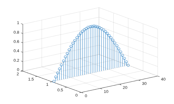
stem3 plots elements of Z against the same y value at equally space x values.

Column Vector Input

Create a 3-D stem plot of cosine values between $$-\pi /2$$ and $$\pi /2$$ with a column vector input.

figure
X = linspace(-pi/2,pi/2,40)';
Z = cos(X);
stem3(Z)

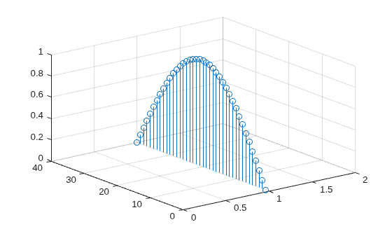
stem3 plots elements of Z against the same x value at equally space y values.

Matrix Input

Create a 3-D stem plot of sine and cosine values between $$-\pi /2$$ and $$\pi /2$$ with a matrix input.

figure
X = linspace(-pi/2,pi/2,40);
Z = [sin(X); cos(X)];
stem3(Z)

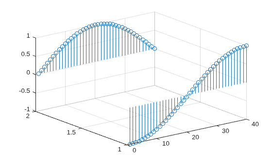
stem3 plots each row of Z against the same y value at equally space x values.

Specify Stem Locations with Vector Inputs

Create a 3-D stem plot and specify the stem locations along a curve. Use view to adjust the angle of the axes in the figure.

figure
X = linspace(-5,5,60);
Y = cos(X);
Z = X.^2;
stem3(X,Y,Z)
view(-8,30)

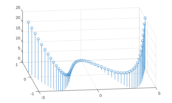
X and Y determine the stem locations. Z determines the marker heights.

Specify Stem Locations with Matrix Inputs

Create a 3-D stem plot with matrix data and specify the stem locations in the xy-plane.

figure
[X,Y] = meshgrid(0:.1:1);
Z = exp(X+Y);
stem3(X,Y,Z)

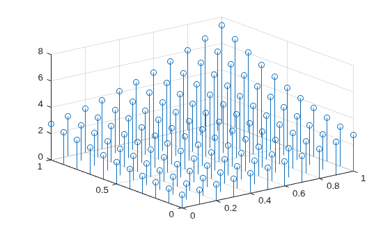
X and Y determine the stem locations. Z determines the marker heights.

Fill in Markers

Create a 3-D stem plot of cosine values between $$-\pi$$ and $$\pi$$ and fill in the markers.

X = linspace(-pi,pi,40);
Z = cos(X);
stem3(Z,'filled')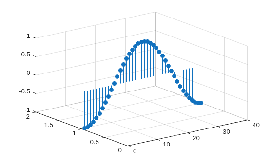

Line Style, Marker Symbol, and Color Options

Create a 3-D stem plot of cosine values between $$-\pi$$ and $$\pi$$. Use a dashed line style for the stem, set the marker symbols to stars, and set the color to magenta.

figure
X = linspace(-pi,pi,40);
Z = cos(X);
stem3(Z,'--*m')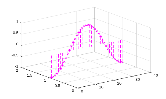

To specify only two of the three LineSpec options, omit the third option from the character vector. For example, '*m' sets the marker symbol and the color and uses the default line style.

Line Style, Marker Symbol, and Color Options

Create a 3-D stem plot and specify the stem locations along a circle. Set the stem to a dotted line style, the marker symbols to stars, and the color to magenta.

figure
theta = linspace(0,2*pi);
X = cos(theta);
Y = sin(theta);
Z = theta;
stem3(X,Y,Z,':*m')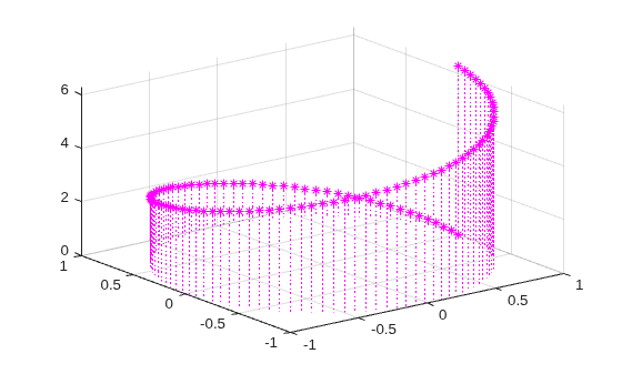

X and Y determine the stem locations. Z determines the marker heights.

Additional Style Options

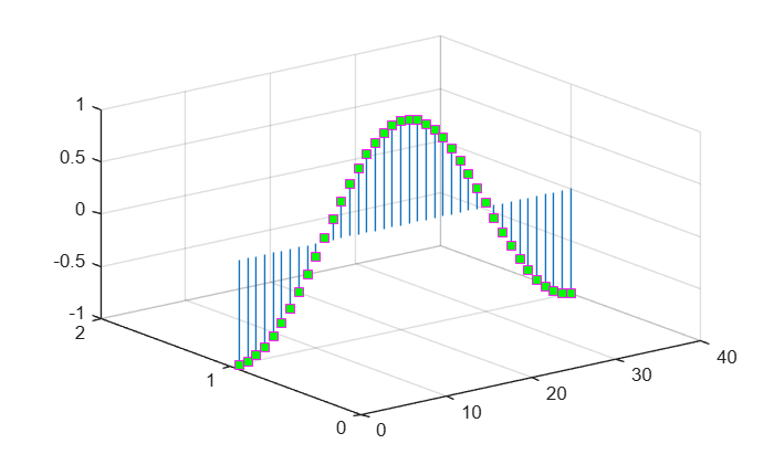
Create a 3-D stem plot of cosine values between $$-\pi$$ and $$\pi$$. Set the marker symbols to squares with green faces and magenta edges.

X = linspace(-pi,pi,40);
Z = cos(X);
stem3(Z,Marker="s",MarkerEdgeColor="m",MarkerFaceColor="g")

Plot Data from a Table

Since R2022b

A convenient way to plot data from a table is to pass the table to the stem3 function and specify the variables to plot.

Read weather.csv as a timetable tbl. Then display the first three rows of the table.

tbl = readtimetable("weather.csv");
head(tbl,3)

            Time            WindDirection    WindSpeed    Humidity    Temperature    RainInchesPerMinute    CumulativeRainfall    PressureHg    PowerLevel    LightIntensity
    ____________________    _____________    _________    ________    ___________    ___________________    __________________    __________    __________    ______________

    25-Oct-2021 00:00:09         46               1          84          49.2                 0                     0               29.96          4.14             0       
    25-Oct-2021 00:01:09         45             1.6          84          49.2                 0                     0               29.96         4.139             0       
    25-Oct-2021 00:02:09         36             2.2          84          49.2                 0                     0               29.96         4.138             0       

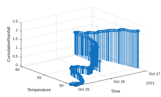
Plot the Time variable on the x-axis, the Temperature variable on the y-axis, and the CumulativeRainfall variable on the z-axis. Return the Stem object as h. Notice that the axis labels match the table variable names.

h = stem3(tbl,"Time","Temperature","CumulativeRainfall");

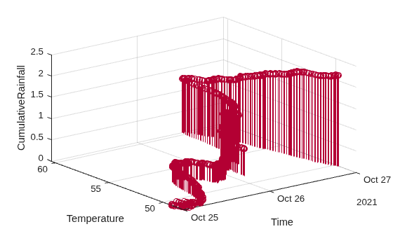
Change the color of the plot to a shade of red by setting the Color property.

h.Color = [0.7 0 0.2];

Plot Multiple Table Variables

Since R2026b

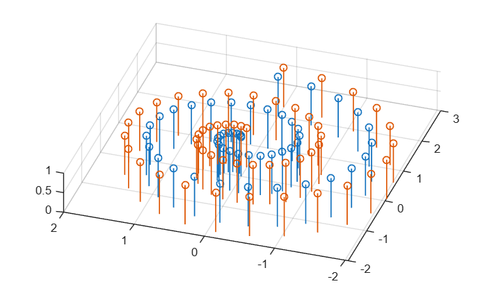
Create two sets of x, y, and z data containing the coordinates of two spirals. Then create a table from the data.

nTurns = 2;        
nPoints = 50;     
t = linspace(0,2*pi*nTurns,nPoints)';  
r = linspace(0,2,nPoints)'; 

X1 = r .* cos(t);
Y1 = r .* sin(t);
Z1 = ones(size(r));

r2 = r + 0.3;
X2 = r2 .* cos(t);
Y2 = r2 .* sin(t);
Z2 = ones(size(r2));
tbl = table(X1,X2,Y1,Y2,Z1,Z2);

Plot the two spirals, and use the view function to view the plot from a higher elevation.

stem3(tbl,["X1","X2"],["Y1","Y2"],["Z1","Z2"],LineWidth=1)
view([-72 76])

Stem Plot in Specific Axes

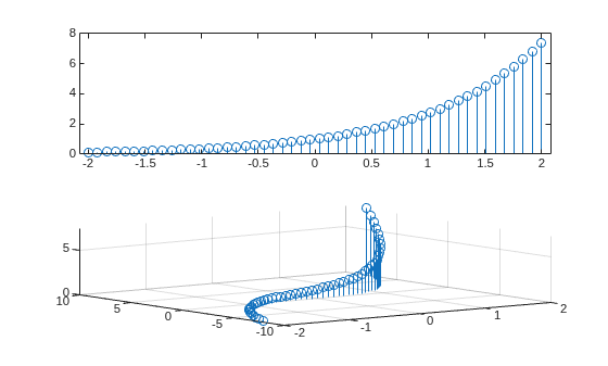
You can display a tiling of plots using the tiledlayout and nexttile functions. Call the tiledlayout function to create a 2-by-1 tiled chart layout. Call the nexttile function to create the axes objects ax1 and ax2. Create separate stem plots in the axes by specifying the axes object as the first argument to stem3.

X = linspace(-2,2,50);
Y = X.^3;
Z = exp(X);
tiledlayout(2,1)

% Top plot
ax1 = nexttile;
stem(ax1,X,Z)

% Bottom plot
ax2 = nexttile;  
stem3(ax2,X,Y,Z)

Modify Stem Series After Creation

Create a 3-D stem plot and return the stem series object.

X = linspace(0,2);
Y = X.^3;
Z = exp(X).*cos(Y);
h = stem3(X,Y,Z,"filled");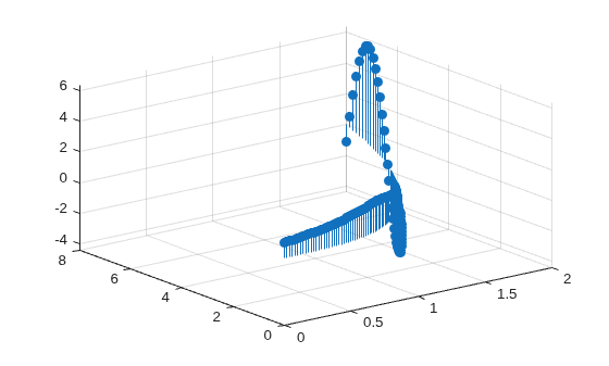

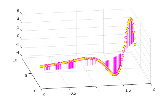
Change the color to magenta and set the marker face color to yellow. Use view to adjust the angle of the axes in the figure. Use dot notation to set properties.

h.Color = "m";
h.MarkerFaceColor = "y";
view(-10,35)

Input Arguments

Z — Data sequence to display

vector or matrix

Data sequence to display, specified as a vector or matrix. stem3 plots each element in Z as a stem extending from the xy-plane and terminating at the data value.

• If Z is a row vector, stem3 plots all elements against the same y value at equally spaced x values.

• If Z is a column vector, stem3 plots all elements against the same x value at equally spaced y values.

• If Z is a matrix, stem3 plots each row of Z against the same y value at equally spaced x values.

Data Types: single | double | int8 | int16 | int32 | int64 | uint8 | uint16 | uint32 | uint64 | logical | categorical | datetime | duration

X — Locations to plot values of Z

vector or matrix

Locations to plot values of Z, specified as a vector or a matrix. Inputs X, Y and Z must be vectors or matrices of the same size.

Data Types: single | double | int8 | int16 | int32 | int64 | uint8 | uint16 | uint32 | uint64 | logical | categorical | datetime | duration

Y — Locations to plot values of Z

vector or matrix

Locations to plot values of Z, specified as a vector or a matrix. Inputs X, Y and Z must be vectors or matrices of the same size.

Data Types: single | double | int8 | int16 | int32 | int64 | uint8 | uint16 | uint32 | uint64 | logical | categorical | datetime | duration

LineSpec — Line style, marker, and color

string scalar | character vector

Line style, marker, and color, specified as a string scalar or character vector containing symbols. The symbols can appear in any order. You do not need to specify all three characteristics (line style, marker, and color). For example, if you omit the line style and specify the marker, then the plot shows only the marker and no line.

Example: "--or" is a red dashed line with circle markers.

Line Style	Description	Resulting Line
"-"	Solid line
"--"	Dashed line
":"	Dotted line
"-."	Dash-dotted line

Marker	Description	Resulting Marker
"o"	Circle
"+"	Plus sign
"*"	Asterisk
"."	Point
"x"	Cross
"_"	Horizontal line
"|"	Vertical line
"square"	Square
"diamond"	Diamond
"^"	Upward-pointing triangle
"v"	Downward-pointing triangle
">"	Right-pointing triangle
"<"	Left-pointing triangle
"pentagram"	Pentagram
"hexagram"	Hexagram

Color Name	Short Name	RGB Triplet	Appearance
"red"	"r"	[1 0 0]
"green"	"g"	[0 1 0]
"blue"	"b"	[0 0 1]
"cyan"	"c"	[0 1 1]
"magenta"	"m"	[1 0 1]
"yellow"	"y"	[1 1 0]
"black"	"k"	[0 0 0]
"white"	"w"	[1 1 1]

tbl — Source table

table | timetable

Source table containing the data to plot, specified as a table or timetable.

zvar — Table variable containing z-coordinates

table variable index | multiple table variable indices (since R2026b)

Table variable containing the z-coordinates, specified as one or more table variable indices. The variable you specify can contain numeric, logical, categorical, datetime, or duration values. If you specify multiple indices, the corresponding variables must all have the same type.

To specify one or more table variable indices, use any of the following indexing schemes.

Indexing Scheme	Examples
Variable names: A string array, character vector, or cell array. A pattern object.	"A" or 'A' — A variable named A ["A","B"] or {'A','B'} — Two variables named A and B "Var"+digitsPattern(1) — Variables named "Var" followed by a single digit
Variable indices: An index number that refers to the location of a variable in the table. A vector of numbers. A logical vector. Typically, this vector is the same length as the number of variables, but you can omit trailing 0 or false values.	3 — The third variable from the table [2 3] — The second and third variables from the table [false false true] — The third variable
Variable type: A vartype subscript that selects variables of a specified type.	vartype("double") — All the variables containing double values

Example: stem3(tbl,"x1","y1","z1") creates a stem plot from the table variables named x1 (the x-coordinates), y1 (the y-coordinates), and z1 (the z-coordinates).

Example: stem3(tbl,"x","y",["z1","z2"]) creates two stem plots that have the same x- and y-coordinates but different z-coordinates. The z-coordinates are specified as a string vector containing the names of two table variables. (since R2026b)

xvar — Table variable containing x-coordinates

table variable index | multiple table variable indices (since R2026b)

Table variable containing the x-coordinates, specified as one or more table variable indices. The variable you specify can contain numeric, logical, categorical, datetime, or duration values. If you specify multiple indices, the corresponding variables must all have the same type.

To specify one or more table variable indices, use any of the following indexing schemes.

Indexing Scheme	Examples
Variable names: A string array, character vector, or cell array. A pattern object.	"A" or 'A' — A variable named A ["A","B"] or {'A','B'} — Two variables named A and B "Var"+digitsPattern(1) — Variables named "Var" followed by a single digit
Variable indices: An index number that refers to the location of a variable in the table. A vector of numbers. A logical vector. Typically, this vector is the same length as the number of variables, but you can omit trailing 0 or false values.	3 — The third variable from the table [2 3] — The second and third variables from the table [false false true] — The third variable
Variable type: A vartype subscript that selects variables of a specified type.	vartype("double") — All the variables containing double values

Example: stem3(tbl,"x1","y1","z1") creates a stem plot from the table variables named x1 (the x-coordinates), y1 (the y-coordinates), and z1 (the z-coordinates).

Example: stem3(tbl,["x1","x2"],"y","z") creates two stem plots that have the same y- and z-coordinates but different x-coordinates. The x-coordinates are specified as a string vector containing the names of two table variables. (since R2026b)

yvar — Table variable containing y-coordinates

table variable index | multiple table variable indices (since R2026b)

Table variable containing the y-coordinates, specified as one or more table variable indices. The variable you specify can contain numeric, logical, categorical, datetime, or duration values. If you specify multiple indices, the corresponding variables must all have the same type.

To specify one or more table variable indices, use any of the following indexing schemes.

Indexing Scheme	Examples
Variable names: A string array, character vector, or cell array. A pattern object.	"A" or 'A' — A variable named A ["A","B"] or {'A','B'} — Two variables named A and B "Var"+digitsPattern(1) — Variables named "Var" followed by a single digit
Variable indices: An index number that refers to the location of a variable in the table. A vector of numbers. A logical vector. Typically, this vector is the same length as the number of variables, but you can omit trailing 0 or false values.	3 — The third variable from the table [2 3] — The second and third variables from the table [false false true] — The third variable
Variable type: A vartype subscript that selects variables of a specified type.	vartype("double") — All the variables containing double values

Example: stem3(tbl,"x1","y1","z1") creates a stem plot from the table variables named x1 (the x-coordinates), y1 (the y-coordinates), and z1 (the z-coordinates).

Example: stem3(tbl,"x",["y1","y2"],"z") creates two stem plots that have the same x- and z-coordinates but different y-coordinates. The y-coordinates are specified as a string vector containing the names of two table variables. (since R2026b)

ax — Axes object

Axes object

Axes object. If you do not specify the axes, then stem plots into the current axes.

Name-Value Arguments

Specify optional pairs of arguments as Name1=Value1,...,NameN=ValueN, where Name is the argument name and Value is the corresponding value. Name-value arguments must appear after other arguments, but the order of the pairs does not matter.

Example: stem3(x,y,z,LineStyle=":") plots the stems as a dotted lines.

The properties listed here are only a subset. For a complete list, see Stem Properties.

LineStyle — Line style

"-" (default) | "--" | ":" | "-." | "none"

Line style, specified as one of the options listed in this table.

Line Style	Description	Resulting Line
"-"	Solid line
"--"	Dashed line
":"	Dotted line
"-."	Dash-dotted line
"none"	No line	No line

LineWidth — Line width of stem and marker edge

0.5 (default) | positive value

Line width of stem and marker edge, specified as a positive value in point units.

Color — Stem color

color name or short name | RGB triplet | hexadecimal color code

Stem color, specified as one of these values:

• Color name (or short name) — Specify any of these values: "red" (or "r"), "green" (or "g"), "blue" (or "b"), "cyan" (or "c"), "magenta" (or "m"), "yellow" (or "y"), "black" (or "k"), or "white" (or "w").

• RGB triplet — Specify the red, green, and blue components of a color as decimal values. An RGB triplet is a three-element row vector whose elements specify the intensities of the red, green, and blue components of the color. The intensities must be in the range [0,1]; for example, [0.4 0.6 0.7].

• Hexadecimal color code — Specify the red, green, and blue components of a color as hexadecimal values. A hexadecimal color code is a character vector or a string scalar that starts with a hash symbol (#) followed by three or six hexadecimal digits, which can range from 0 to F. The values are not case sensitive. The color codes "#FF8800", "#ff8800", "#F80", and "#f80" are equivalent.

This table shows the default color palettes for plots in the light and dark themes. You can get the RGB triplets and hexadecimal color codes for these palettes using the orderedcolors and rgb2hex functions. For example, get the RGB triplets for the "gem" palette and convert them to hexadecimal color codes.

RGB = orderedcolors("gem");
H = rgb2hex(RGB);

Before R2024a: Get the hexadecimal color codes using H = compose("#%02X%02X%02X",round(RGB*255)).

Before R2023b: Get the RGB triplets using RGB = get(groot,"FactoryAxesColorOrder").

Palette	Palette Colors
"gem" — Light theme default Before R2025a: Most plots use these colors by default.
"glow" — Dark theme default

Example: stem3(x,y,z,Color="blue") specifies blue stems using a color name.

Example: stem3(x,y,z,Color=[0 0 1]) specifies blue stems using an RGB triplet.

Example: stem3(x,y,z,Color="#0000FF") specifies blue stems using a hexadecimal color code.

Marker — Marker symbol

"o" (default) | "+" | "*" | "." | "x" | ...

Marker symbol, specified as one of the markers listed in this table.

Marker	Description	Resulting Marker
"o"	Circle
"+"	Plus sign
"*"	Asterisk
"."	Point
"x"	Cross
"_"	Horizontal line
"|"	Vertical line
"square"	Square
"diamond"	Diamond
"^"	Upward-pointing triangle
"v"	Downward-pointing triangle
">"	Right-pointing triangle
"<"	Left-pointing triangle
"pentagram"	Pentagram
"hexagram"	Hexagram
"none"	No markers	Not applicable

Example: stem3(x,y,z,Marker="+") specifies plus sign markers.

Example: stem3(x,y,z,Marker="diamond") specifies diamond markers.

MarkerSize — Marker size

6 (default) | positive value

Marker size, specified as a positive value in points, where 1 point = 1/72 of an inch.

MarkerEdgeColor — Marker outline color

"auto" (default) | colorname or short name | RGB triplet | hexadecimal color code

Marker outline color, specified as one of these values:

• "auto" — Use the value of the Color property.

• Color name (or short name) — Specify any of these values: "red" (or "r"), "green" (or "g"), "blue" (or "b"), "cyan" (or "c"), "magenta" (or "m"), "yellow" (or "y"), "black" (or "k"), or "white" (or "w").

• RGB triplet — Specify the red, green, and blue components of a color as decimal values. An RGB triplet is a three-element row vector whose elements specify the intensities of the red, green, and blue components of the color. The intensities must be in the range [0,1]; for example, [0.4 0.6 0.7].

• Hexadecimal color code — Specify the red, green, and blue components of a color as hexadecimal values. A hexadecimal color code is a character vector or a string scalar that starts with a hash symbol (#) followed by three or six hexadecimal digits, which can range from 0 to F. The values are not case sensitive. The color codes "#FF8800", "#ff8800", "#F80", and "#f80" are equivalent.

This table shows the default color palettes for plots in the light and dark themes. You can get the RGB triplets and hexadecimal color codes for these palettes using the orderedcolors and rgb2hex functions. For example, get the RGB triplets for the "gem" palette and convert them to hexadecimal color codes.

RGB = orderedcolors("gem");
H = rgb2hex(RGB);

Before R2024a: Get the hexadecimal color codes using H = compose("#%02X%02X%02X",round(RGB*255)).

Before R2023b: Get the RGB triplets using RGB = get(groot,"FactoryAxesColorOrder").

Palette	Palette Colors
"gem" — Light theme default Before R2025a: Most plots use these colors by default.
"glow" — Dark theme default

MarkerFaceColor — Marker fill color

"none" (default) | "auto" | color name or short name | RGB triplet | hexadecimal color code

Marker fill color, specified as one of these values:

• "none" — Do not fill the markers with any color.

• "auto" — Use an invisible plot box and fill the markers with the figure color to provide a transparent look.

• Color name (or short name) — Specify any of these values: "red" (or "r"), "green" (or "g"), "blue" (or "b"), "cyan" (or "c"), "magenta" (or "m"), "yellow" (or "y"), "black" (or "k"), or "white" (or "w").

• RGB triplet — Specify the red, green, and blue components of a color as decimal values. An RGB triplet is a three-element row vector whose elements specify the intensities of the red, green, and blue components of the color. The intensities must be in the range [0,1]; for example, [0.4 0.6 0.7].

• Hexadecimal color code — Specify the red, green, and blue components of a color as hexadecimal values. A hexadecimal color code is a character vector or a string scalar that starts with a hash symbol (#) followed by three or six hexadecimal digits, which can range from 0 to F. The values are not case sensitive. The color codes "#FF8800", "#ff8800", "#F80", and "#f80" are equivalent.

This table shows the default color palettes for plots in the light and dark themes. You can get the RGB triplets and hexadecimal color codes for these palettes using the orderedcolors and rgb2hex functions. For example, get the RGB triplets for the "gem" palette and convert them to hexadecimal color codes.

RGB = orderedcolors("gem");
H = rgb2hex(RGB);

Before R2024a: Get the hexadecimal color codes using H = compose("#%02X%02X%02X",round(RGB*255)).

Before R2023b: Get the RGB triplets using RGB = get(groot,"FactoryAxesColorOrder").

Palette	Palette Colors
"gem" — Light theme default Before R2025a: Most plots use these colors by default.
"glow" — Dark theme default

Output Arguments

h — Stem object

Stem

Stem object. This is a unique identifier, which you can use to modify the properties of the Stem object after it is created.

Extended Capabilities

GPU Arrays

Accelerate code by running on a graphics processing unit (GPU) using Parallel Computing Toolbox™.

The stem3 function supports GPU array input with these usage notes and limitations:

• This function accepts GPU arrays, but does not run on a GPU.

For more information, see Run MATLAB Functions on a GPU (Parallel Computing Toolbox).

Distributed Arrays

Partition large arrays across the combined memory of your cluster using Parallel Computing Toolbox™.

The stem3 function supports distributed arrays with these usage notes and limitations:

• This function operates on distributed arrays, but executes on the client MATLAB^®.

For more information, see Run MATLAB Functions with Distributed Arrays (Parallel Computing Toolbox).

Version History

Introduced before R2006a

R2026b: Plot multiple table variables simultaneously

Create 3-D stem plots from multiple table variables simultaneously by passing a table to the stem3 function followed by the table variables you want to plot. For an example, see Plot Multiple Table Variables.

R2022b: Expanded data type support

The x, y, and z input arguments can be any numeric, logical, datetime, duration, or categorical values. In previous releases, only numeric and logical values were supported.

R2022b: Pass tables directly to stem3

Create plots by passing a table to the stem3 function followed by the variables you want to plot. When you specify your data as a table, the axis labels and the legend (if present) are automatically labeled using the table variable names.