Replace Discouraged Instances of hist and histc

Old Histogram Functions (`hist`, `histc`)

Earlier versions of MATLAB^® use the hist and histc functions as the primary way to create histograms and calculate histogram bin counts. These functions, while good for some general purposes, have limited overall capabilities. The use of hist and histc in new code is discouraged for these reasons (among others):

After using hist to create a histogram, modifying properties of the histogram is difficult and requires recomputing the entire histogram.
The default behavior of hist is to use 10 bins, which is not suitable for many data sets.
Plotting a normalized histogram requires manual computations.
hist and histc do not have consistent behavior.

Recommended Histogram Functions

The histogram, histcounts, and discretize functions dramatically advance the capabilities of histogram creation and calculation in MATLAB, while still promoting consistency and ease of use. histogram, histcounts, and discretize are the recommended histogram creation and computation functions for new code.

Of particular note are the following changes, which stand as improvements over hist and histc:

histogram can return a histogram object. You can use the object to modify properties of the histogram.
Both histogram and histcounts have automatic binning and normalization capabilities, with several common options built-in.
histcounts is the primary calculation function for histogram. The result is that the functions have consistent behavior.
discretize provides additional options and flexibility for determining the bin placement of each element.

Differences Requiring Code Updates

Despite the aforementioned improvements, there are several important differences between the old and now recommended functions, which might require updating your code. The tables summarize the differences between the functions and provide suggestions for updating code.

Code Updates for hist

Difference	Old behavior with `hist`	New behavior with `histogram`
Input matrices	`hist` creates a histogram for each column of an input matrix and plots the histograms side-by-side in the same figure. A = randn(100,2); hist(A)	`histogram` treats the input matrix as a single tall vector and creates a single histogram. To plot multiple histograms, create a different histogram object for each column of data. Use the `hold on` command to plot the histograms in the same figure. A = randn(100,2); h1 = histogram(A(:,1),10) edges = h1.BinEdges; hold on h2 = histogram(A(:,2),edges) The above code example uses the same bin edges for each histogram, but in some cases it is better to set the `BinWidth` of each histogram to be the same instead. Also, for display purposes, it might be helpful to set the `FaceAlpha` property of each histogram, as this affects the transparency of overlapping bars.
Bin specification	`hist` accepts the bin centers as a second input.	`histogram` accepts the bin edges as a second input. To convert bin centers into bin edges for use with `histogram`, see Convert Bin Centers to Bin Edges. Note In cases where the bin centers used with `hist` are integers, such as `hist(A,-3:3)`, use the new built-in binning method of `histogram` for integers. histogram(A,'BinLimits',[-3,3],'BinMethod','integers')
Output arguments	`hist` returns the bin counts as an output argument, and optionally can return the bin centers as a second output argument. A = randn(100,1); [N, Centers] = hist(A)	`histogram` returns a histogram object as an output argument. The object contains many properties of interest (bin counts, bin edges, and so on). You can modify aspects of the histogram by changing its property values. For more information, see `histogram`. A = randn(100,1); h = histogram(A); N = h.Values Edges = h.BinEdges Note To calculate bin counts (without plotting a histogram), replace `[N, Centers] = hist(A)` with `[N,edges] = histcounts(A,nbins)`.
Default number of bins	`hist` uses 10 bins by default.	Both `histogram` and `histcounts` use an automatic binning algorithm by default. The number of bins is determined by the size and spread of the input data. A = randn(100,1); histogram(A) histcounts(A)
Bin limits	`hist` uses the minimum and maximum finite data values to determine the left and right edges of the first and last bar in the plot. `-Inf` and `Inf` are included in the first and last bin, respectively.	If `BinLimits` is not set, then `histogram` uses rational bin limits based on, but not exactly equal to, the minimum and maximum finite data values. `histogram` ignores `Inf` values unless one of the bin edges explicitly specifies `Inf` or `-Inf` as a bin edge. To reproduce the results of `hist(A)` for finite data (no `Inf` values), use 10 bins and explicitly set `BinLimits` to the minimum and maximum data values. A = randi(5,100,1); histogram(A,10,'BinLimits',[min(A) max(A)])

Code Updates for histc

Difference Old behavior with histc New behavior with histcounts

Input matrices

Difference	Old behavior with `histc`	New behavior with `histcounts`
Input matrices	`histc` calculates the bin counts for each column of input data. For an input matrix of size `m`-by-`n`, `histc` returns a matrix of bin counts of size `length(edges)`-by-`n`. A = randn(100,10); edges = -4:4; N = histc(A,edges)	`histcounts` treats the input matrix as a single tall vector and calculates the bin counts for the entire matrix. A = randn(100,10); edges = -4:4; N = histcounts(A,edges) Use a for-loop to calculate bin counts over each column. A = randn(100,10); nbins = 10; N = zeros(nbins, size(A,2)); for k = 1:size(A,2) N(:,k) = histcounts(A(:,k),nbins); end If performance is a problem due to a large number of columns in the matrix, then consider continuing to use `histc` for the column-wise bin counts.
Values included in last bin	`histc` includes an element `A(i)` in the last bin if `A(i) == edges(end)`. The output, `N`, is a vector with `length(edges)` elements containing the bin counts. Values falling outside the bins are not counted.	`histcounts` includes an element `A(i)` in the last bin if `edges(end-1) <= A(i) <= edges(end)`. In other words, `histcounts` combines the last two bins from `histc` into a single final bin. The output, `N`, is a vector with `length(edges)-1` elements containing the bin counts. If you specify the bin edges, then values falling outside the bins are not counted. Otherwise, `histcounts` automatically determines the proper bin edges to use to include all of the data. A = 1:4; edges = [1 2 2.5 3] N = histcounts(A) N = histcounts(A,edges) The last bin from `histc` is primarily useful to count integers. To do this integer counting with `histcounts`, use the `'integers'` bin method: N = histcounts(A,'BinMethod','integers');
Output arguments	`histc` returns the bin counts as an output argument, and optionally can return the bin indices as a second output argument. A = randn(15,1); edges = -4:4; [N,Bin] = histc(A,edges)	For bin count calculations like `N = histc(A,edges)` or `[N,bin] = histc(A,edges)`, use `histcounts`. The `histcounts` function returns the bin counts as an output argument, and optionally can return the bin edges as a second output, or the bin indices as a third output. A = randn(15,1); [N,Edges,Bin] = histcounts(A) For bin placement calculations like `[~,Bin] = histc(A,edges)`, use `discretize`. The `discretize` function offers additional options for determining the bin placement of each element. A = randn(15,1); edges = -4:4; Bin = discretize(A,edges)

histc calculates the bin counts for each column of input data. For an input matrix of size m-by-n, histc returns a matrix of bin counts of size length(edges)-by-n.

A = randn(100,10);
edges = -4:4;
N = histc(A,edges)

histcounts treats the input matrix as a single tall vector and calculates the bin counts for the entire matrix.

A = randn(100,10);
edges = -4:4;
N = histcounts(A,edges)

Use a for-loop to calculate bin counts over each column.

A = randn(100,10);
nbins = 10;
N = zeros(nbins, size(A,2));
for k = 1:size(A,2)
   N(:,k) = histcounts(A(:,k),nbins);
end

If performance is a problem due to a large number of columns in the matrix, then consider continuing to use histc for the column-wise bin counts.

Values included in last bin

histc includes an element A(i) in the last bin if A(i) == edges(end). The output, N, is a vector with length(edges) elements containing the bin counts. Values falling outside the bins are not counted.

histcounts includes an element A(i) in the last bin if edges(end-1) <= A(i) <= edges(end). In other words, histcounts combines the last two bins from histc into a single final bin. The output, N, is a vector with length(edges)-1 elements containing the bin counts. If you specify the bin edges, then values falling outside the bins are not counted. Otherwise, histcounts automatically determines the proper bin edges to use to include all of the data.

A = 1:4;
edges = [1 2 2.5 3]
N = histcounts(A)
N = histcounts(A,edges)

The last bin from histc is primarily useful to count integers. To do this integer counting with histcounts, use the 'integers' bin method:

N = histcounts(A,'BinMethod','integers');

Output arguments

histc returns the bin counts as an output argument, and optionally can return the bin indices as a second output argument.

A = randn(15,1);
edges = -4:4;
[N,Bin] = histc(A,edges)

For bin count calculations like N = histc(A,edges) or [N,bin] = histc(A,edges), use histcounts. The histcounts function returns the bin counts as an output argument, and optionally can return the bin edges as a second output, or the bin indices as a third output.
```
A = randn(15,1);
[N,Edges,Bin] = histcounts(A)
```
For bin placement calculations like [~,Bin] = histc(A,edges), use discretize. The discretize function offers additional options for determining the bin placement of each element.
```
A = randn(15,1);
edges = -4:4;
Bin = discretize(A,edges)
```

Convert Bin Centers to Bin Edges

Open Live Script

The hist function accepts bin centers, whereas the histogram function accepts bin edges. To update code to use histogram, you might need to convert bin centers to bin edges to reproduce results achieved with hist.

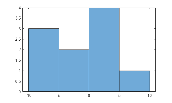
For example, specify bin centers for use with hist. These bins have a uniform width.

A = [-9 -6 -5 -2 0 1 3 3 4 7];
centers = [-7.5 -2.5 2.5 7.5];
hist(A,centers)

Figure contains an axes object. The axes object contains an object of type patch. This object represents A.

To convert the bin centers into bin edges, calculate the midpoint between consecutive values in centers. This method reproduces the results of hist for both uniform and nonuniform bin widths.

d = diff(centers)/2;
edges = [centers(1)-d(1), centers(1:end-1)+d, centers(end)+d(end)];

The hist function includes values falling on the right edge of each bin (the first bin includes both edges), whereas histogram includes values that fall on the left edge of each bin (and the last bin includes both edges). Shift the bin edges slightly to obtain the same bin counts as hist.

edges(2:end) = edges(2:end)+eps(edges(2:end))

edges = 1×5

  -10.0000   -5.0000    0.0000    5.0000   10.0000

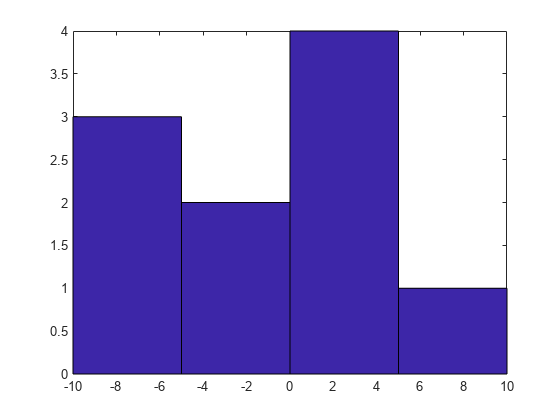
Now, use histogram with the bin edges.

histogram(A,edges)

Figure contains an axes object. The axes object contains an object of type histogram.