Reduced Order Modeling of a Nonlinear Dynamical System using Neural State-Space Model with Autoencoder

This example shows reduced order modeling of a nonlinear dynamical system using a neural state-space (NSS) modeling technique. The nonlinear system used to describe the approach is a cascade of nonlinear mass-spring-damper (MSD) systems. The development of the reduced order model hinges on training a neural network with three parts:

1. The encoder network that maps the data into a low-dimensional space

2. The state network that learns the dynamics in the encoded space

3. The decoder network that maps the data back to the original space

The Simulink® model used to collect data is introduced in Reduced Order Modeling of a Nonlinear Dynamical System as an Identified Linear Parameter Varying Model example.

You select 25 masses, resulting in a state dimension of 50, where the first 25 states, $$x$$, represent the location of each mass, and the next 25 states, $$\underset{}{\overset{\dot{}}{x}}$$, represent the velocity of each mass. The nonlinearity is in the stiffness of each spring, $$k(x)=k_{1}x+k_2{x}^3$$. You excite the system with no external disturbance ($$F=0$$) and subject it to a random stair-step input $$u$$. You collect all the states, both positions $$x$$ and velocities $$\underset{}{\overset{\dot{}}{x}}$$, and treat this combined state vector as the output $$y$$. The objective is to identify a neural state-space model that employs an autoencoder to encapsulate these nonlinear dynamics effectively.

Data Preparation

Set the values of the parameters required to simulate the MSD system. You set the number of masses $\mathit{M}=25$, the mass of individual blocks $\mathit{m}=1\mathrm{kg}$, linear spring constant ${\mathit{k}}_1=0.5\mathit{N}/\mathit{m}$, cubic spring constant ${\mathit{k}}_2=1$${\mathit{N}/\mathit{m}}^3$, linear damping constant ${\mathit{b}}_1=1N/(m/s)$, and cubic damping constant ${\mathit{b}}_2=0.1\mathit{N}/{\left(\mathit{m}/\mathit{s}\right)}^3$.

rng default
M = 25;
m = 1;
k1 = 0.5;
k2 = 1;
b1 = 1;
b2 = 0.1;

Experimental Setup

You generate two random stair-step inputs using the helper function stairInputs defined at the end of the example. You use the first one to train the model and the second for validation.

Nt = 1000;   % number of samples
Nu = 2;      % number of input sequences
for i = 1:Nu
   [u{i},tin] = stairInputs(Nt);
end

All masses are at rest in the beginning. You excite them using inputs and start the oscillation.

ic = zeros(2*M,1);  
Tf = tin(end);
dt = tin(2) - tin(1);

% Initial condition for Simulink model (needed to update the size of x in MSD_NL)
F = 0;
U0 = 0;
dFt = [0, 0; Tf, 0];

Collect data by simulating the Simulink model.

dXall = zeros(2*M,Nt,Nu);
dUall = zeros(1,Nt,Nu);

for i=1:Nu
   x0 = ic;
   uin = u{i};
   dut = [tin(:) uin(:)];
   simout_NL = sim('MSD_NL');
   states = simout_NL.simout.Data;
   states = squeeze(states);

   dXall(:,:,i) = states;
   dUall(:,:,i) = uin;
end

X = permute(dXall,[2,1,3]);
U = permute(dUall,[2,1,3]);
X = squeeze(mat2cell(X,Nt,2*M,ones(1,Nu)));
U = squeeze(mat2cell(U,Nt,1,ones(1,Nu)));

zt = iddata(X{1}, U{1}, Ts=dt, Tstart=0); % training data

zv = iddata(X{2}, U{2}, Ts=dt, Tstart=0); % validation data

Data Display

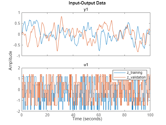
Display the input and the ${\mathit{i}}^{\mathrm{th}}$ state of estimation and validation data.

i =25;
z_training = zt;
z_training.y = z_training.y(:,i);
z_validation = zv;
z_validation.y = z_validation.y(:,i);
idplot(z_training,z_validation)
legend

By playing with the spinner, you can notice that for i = 1 to 20 and i = 26 to 45, the value of the state is very small. This corresponds to the physical law, since those states represent the leftmost masses which are barely affected by the force on the rightmost mass. This also suggests that only the five rightmost masses carry most of the energy. So choose to reduce the model order to 10 (two states from each of the five components).

NSS Model Estimation

You first create the NSS object, its state network, encoder network, and decoder network used for training. Set the LatentDim property of the idNeuralStateSpace object to 10, as you are reducing the model order to 10.

rng default
nx = 50;
nu = 1;
nd = 10;
nss = idNeuralStateSpace(nx,NumInputs=nu,LatentDim=nd);
nss.StateNetwork = createMLPNetwork(nss,'state',...
   LayerSizes=[128 128],Activations="tanh");
nss.Encoder = createMLPNetwork(nss,'encoder',...
   LayerSizes=[128 128], Activations="tanh");
nss.Decoder = createMLPNetwork(nss,'decoder',...
   LayerSizes=[128 128],Activations="tanh");

Specify training options using nssTrainingOptions.

opt = nssTrainingOptions('adam');
opt.LearnRate = 0.0015;
opt.MaxEpochs = 100;
opt.MiniBatchSize = 800;
opt.WindowSize = 40;
opt.Overlap = 39;

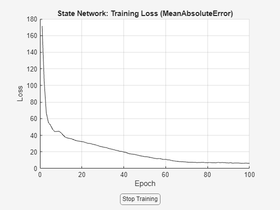
Train the model using nlssest.

warnState = warning('off','Ident:estimation:NparGTNsamp');
cleanupObj = onCleanup(@()warning(warnState));
sys = nlssest(zt,nss,opt);

Generating estimation report...done.

clear("cleanupObj");

NSS Model Validation

Validate the model and calculate the mean-squared error between the validation data and simulation outputs.

zy = sim(sys,zv);
MSE = goodnessOfFit(zv.y,zy.y,'MSE')

MSE = 
0.0040

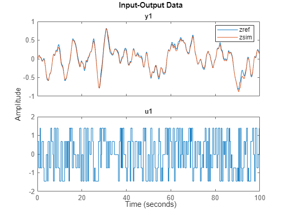
Display the validation data and simulation result of the ${\mathit{j}}^{\mathrm{th}}$ state.

j = 25;
zref = zv;    % validation data
zref.y = zref.y(:,j);
zsim = zy;    % simulation result
zsim.Name = '';
zsim.y = zsim.y(:,j);   
idplot(zref,zsim)
legend

mdl = 'MSD_NSS';
open_system(mdl)
sim(mdl);

Note that the simulation result on the left 20 masses is not good since those values are too small and neglected during the estimation phase. To learn dynamics on those states, you can increase the latent dimension of the encoder and/or normalize the data for training (which gives equal emphasis on the errors corresponding to each state).

Function to Generate Random Stair-Step Signal

function [stairSignal, t] = stairInputs(L)
stepHeights = randi([1, 5], 1, L); % Random step heights between 1 and 5

rng default 
stepWidths = randi([2, 6], 1, L); % Random step widths between 2 and 6

stairSignal = repelem(stepHeights, stepWidths);
stairSignal = normalize(stairSignal);
stairSignal = stairSignal(1:L);
t = 0:(length(stairSignal) - 1);
t = t/10;
end