Reduced Order Model of an Airframe

This example shows how to create a reduced order model (ROM) of an airframe modeled in Simulink® using a discrete-time neural state-space (NSS) model. You can then use the trained model as a virtual sensor or as a prediction model in model predictive control, either of which can be deployed to hardware.

In this example, you use the Reduced Order Modeler app to:

• Specify ROM inputs and outputs.

• Design experiments.

• Generate input and output data from the Simulink model.

• Train an AI-based surrogate model from the input and output data using preconfigured training templates.

• Implement the trained model in Simulink.

This example requires the Reduced Order Modeler for MATLAB® add-on and the Aerospace Blockset™ toolbox software. You can install the add-on using the instructions in Get and Manage Add-Ons.

For more information on reduced order modeling, see Reduced Order Modeling (Simulink).

Open Model and Reduced Order Modeler App

The Simulink model airframe describes the pitch axis dynamics of an airframe over a range of operating conditions. The model includes the earth coordinates $$(X_e,Z_e)$$, the body coordinates $$(u,w)$$, the pitch angle $$\theta$$, and the pitch rate $$q=\underset{}{\overset{\dot{}}{\theta }}$$. This figure summarizes the relationship between the inertial and body frames, the flight path angle $$\gamma$$, the incidence angle $$\alpha$$, and the pitch angle $$\theta$$.

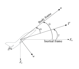
The airframe dynamics are nonlinear and the aerodynamic forces and moments depend on the speed $$V$$ (which is not shown at the top level of the model) and incidence $$\alpha$$. The model simulates a scenario with constant thrust along the body frame ($\mathit{u}$-axis) and includes a fin deflection input $$\delta$$. The model outputs the incidence angle $$\alpha$$, the acceleration along the body frame $$Ax$$, the acceleration perpendicular to the body frame $$Az$$, and the pitch rate $$q=\underset{}{\overset{\dot{}}{\theta }}$$.

Open the Simulink model and run a baseline simulation.

open_system("airframe")
sim("airframe")

To capture the system dynamics from $$\delta$$, to $$\alpha$$, $$Ax$$, $$Az$$, and $$q$$, create an NSS model. First, open the Reduced Order Modeler app.

reducedOrderModeler("airframe")

This example describes the complete workflow to create a ROM. However, you can choose to begin at the Run Experiment step or the Create ROM Using Discrete-Time NSS Model step by loading the session files mentioned in these steps. These session files provide the same results as if you had completed the steps up to that point. To use a ROM that was pretrained by following the steps in this example, begin at the Use Trained NSS Model in Simulink step.

Select ROM Inputs and Outputs

Specify the ROM inputs and outputs.

• In the app, on the Reduced Order Model tab, click New Session. The Select ROM I/Os dialog box opens.

• In the Select ROM I/Os dialog box, click Select Signals. The Simulink model appears in a mode where you can interact with it and select signals.

• To select a signal, click it in the model and then select it in the list that appears. Select the signals delta, alpha, ax, q, and az.

• In the Select ROM I/Os dialog box, change the I/O Type of the alpha, ax, q, and az signals to ROM Output. Keep the I/O Type of the delta signal as the default type, ROM & Simulation Input. Specifying delta as a ROM and simulation input allows you to collect data from simulations using different delta signal values.

• Click Select Parameters. The Simulink model appears in a mode where you can interact with it and select parameters.

• To select a parameter, click the block and then select the parameter from the list that appears. Select the parameters alpha_ini, q_ini, theta_ini, and v_ini. These parameters are used in the airframe/Airframe Model/Aerodynamics & Equations of Motion/3DOF (Body Axes) block to set the initial conditions of the model.

• Change the I/O Type of all the parameters to Simulation Input. Specifying the alpha_ini, q_ini, theta_ini, v_ini parameters as simulation inputs allows you to collect data from different combinations of initial conditions.

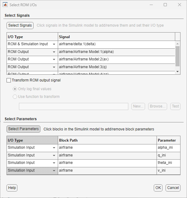
• Click OK. The selected inputs, parameters, and outputs appear in the Inputs/Outputs pane in the Reduced Order Modeler app.

Configure Experiment

Configure experiments to generate data for training the ROM. First, specify how to vary the delta signal:

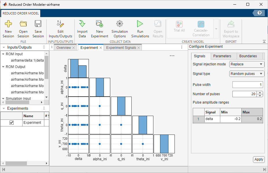
• On the Reduced Order Model tab, click New Experiment. The Experiment and Experiment Signals tabs open. By default, the name of this experiment is Experiment.

• In the Configure Experiment pane, on the Signals tab, specify the experiment settings for delta. Choose the Signal injection mode as Replace, which means that the pulse sequence replaces the delta signal during the simulation.

• Specify Signal Type, Pulse width, and Number of pulses as Random pulses, 1, and 20, respectively. Random pulses specifies that the app selects signal perturbations at random within the signal range.

• In the baseline simulation you ran, the delta signal varies mostly within the range -0.2 to +0.2. So, set the delta Min value as -0.2 and the Max value as 0.2.

Next, specify how to vary the parameters:

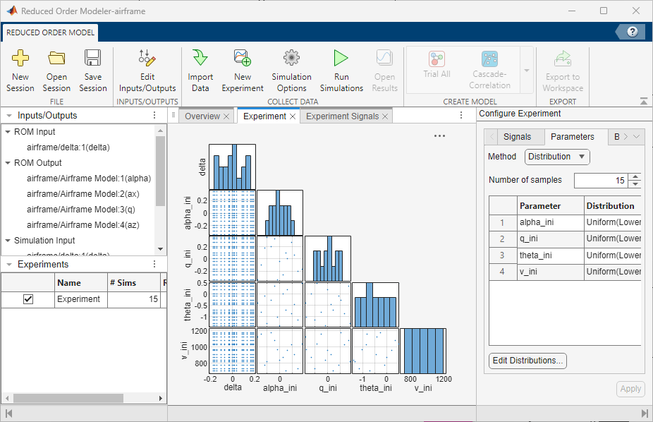
• On the Parameters tab, choose Method as Distribution.

• To specify the distribution from which to sample the parameter values, click Edit Distributions.

• In the Edit Distributions dialog box, select Sampling Method as Latin Hypercube.

• For each parameter, specify Distribution as Uniform and enter limits based on your knowledge of the physical system. By default, these limits are set to -10% and +10% of the parameter values obtained from a baseline simulation of the model. Click OK.

Parameter	Lower Limit	Upper Limit
alpha_ini	-20*pi/180	20*pi/180
q_ini	-0.4	0.4
theta_ini	-1.5	0.5
v_ini	690	1200

For each simulation in the experiment, the app uses the Latin Hypercube sampling method to choose random values of the parameters within their specified ranges.

• On the Parameters tab, in the Number of samples field, specify 15 and click Apply.

This experiment definition produces 15 simulation runs, that is, one simulation for each combination of parameter values. The different combinations of parameter values represent different initial conditions of the model. Each simulation uses the same random pulse sequence for the delta signal with pulse amplitudes in the range [-0.2 0.2]. This configuration drives the airframe into different operating regions from the initial condition.

On the Experiment tab, a scatter plot shows the relationships between input signals and parameter values.

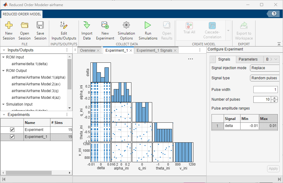
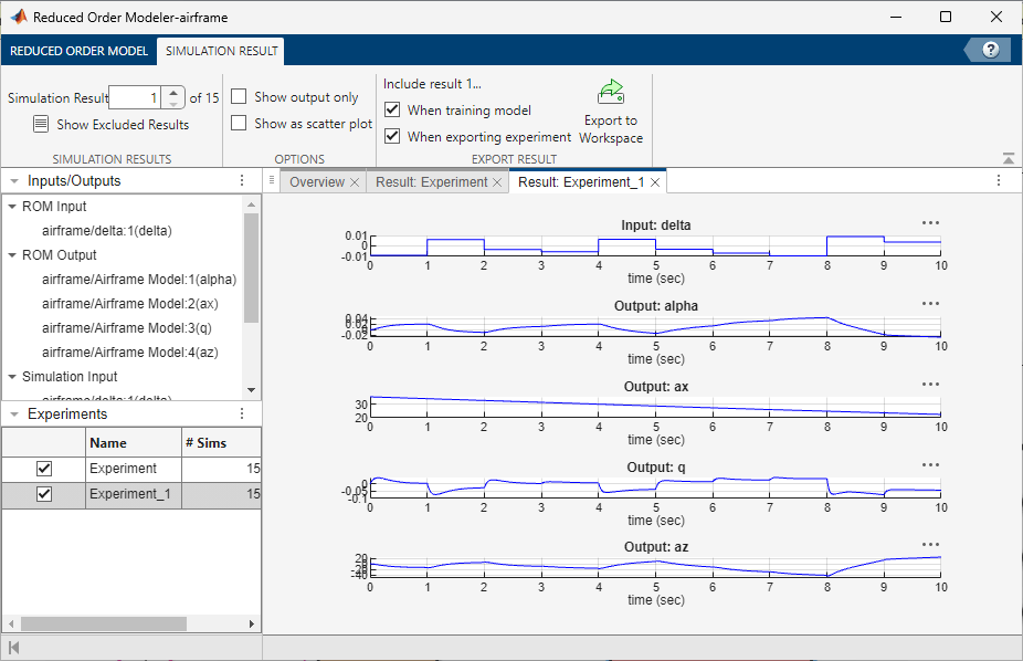
Add a second experiment Experiment_1, where you set the delta signal to a shorter random pulse sequence with smaller amplitudes. Specify Number of pulses as 10 and the delta Min and Max values as -0.01 and 0.01, respectively. Specify the parameter variation as before. This experiment collects more data around the baseline simulation values using small amplitude delta signals.

For more information on the options available to configure experiments, see Configure Options in Reduced Order Modeler (Simulink).

Run Experiment

Note: You can begin at this step by loading the airframe_ROMSession_expsetup.mat session file in the app. This session file includes the same experiment configuration as if you had completed the previous steps in the example. To load the file, on the Reduced Order Model tab, click Open Session, find the session file, and open it. To view the experiment configuration, in the Experiments pane, double-click the experiment.

Log the input, parameter, and output data for training the ROM by running the Simulink model with the experiments you configured.

The two experiments together produce a total of 30 simulations using different combinations of parameter values. If you have Parallel Computing Toolbox™ software, you can run these simulations in parallel:

• On the Reduced Order Model tab, click Simulation Options.

• In the Run Options dialog box, select Use Parallel when running multiple simulations.

• Click OK.

• If the parallel pool is not already enabled, at the MATLAB command line, type parpool('local').

To run the simulations, on the Reduced Order Model tab, click Run Simulations.

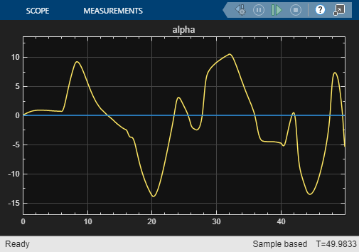
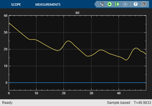
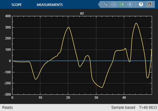
View the simulation results. To choose a simulation result of an experiment to view, click the result tab for that experiment. Then, on the Simulation Result tab, select a simulation number in the Simulation Result box. For example, the Result: Experiment_1 tab shows plots of the input and output signal values from the selected Experiment_1 simulation.

You can skip to this step in the examples by opening the airframe_ROMsession_results.mat session file. To view the simulation results, on the Reduced Model Order tab, click Open Results.

Create ROM Using Discrete-Time NSS Model

Note: You can begin at this step by loading the airframe_ROMSession_results.mat session file in the app. This session file contains simulation data from the airframe model, collected using the same experiment configuration demonstrated in this example. To load the file, on the Reduced Order Model tab, click Open Session, find the session file, and open it. To view the simulation results, on the Reduced Order Model tab, click Open Results.

Create a discrete-time NSS model by using the data you collected from the experiments. First, open the Experiment Manager app:

• On the Reduced Order Model tab, in the Create Model gallery, select Neural State Space as the model type. The Export Results dialog box opens.

• In the Export Results dialog box, select all experiments and ROM input and output signals. Click OK.

• In the Create Experiment dialog box, select New Project, click OK, and save the experiment project. The Experiment Manager app opens.

Experiment Manager creates an experiment to train a discrete-time NSS model using the selected signals and the results of the selected experiments.

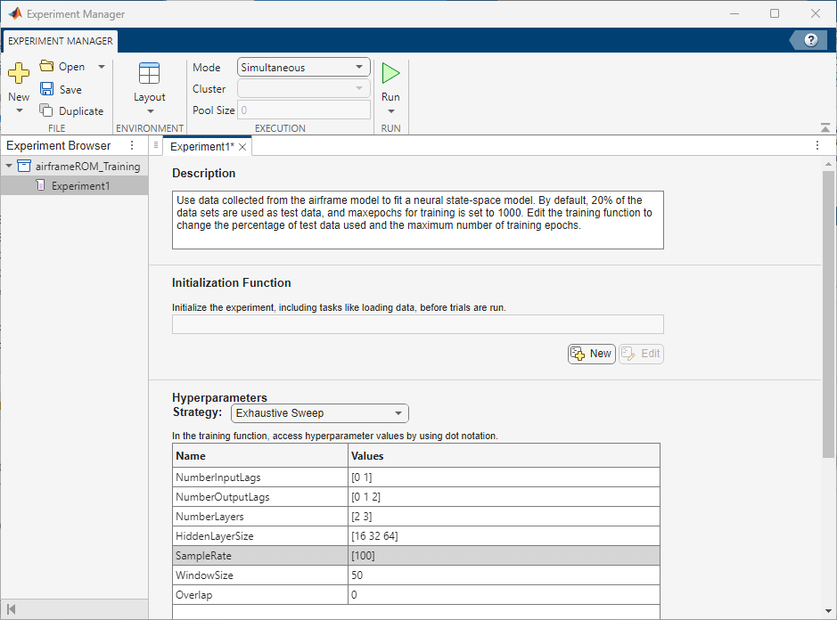
To view experiment information such as the high-fidelity system, ROM model type, and test data percentage in Experiment Manager, view the Description text box on the Experiment1 tab.

Set the Hyperparameters Strategy to Exhaustive Sweep. Experiment Manager sweeps over different hyperparameters to train different models, then determines which models work best. Set the hyperparameters:

• NumberInputLags — [0 1]

• NumberOutputLags — [0 1 2]

• NumberLayers — [2 3]

• HiddenLayerSize — [16 32 64]

• SampleRate — [100]

• WindowSize — 50

• Overlap — 0

The general form of an NSS model is

$$x[k+1]=f(x[k],u[k])$$,

where $\mathit{x}\left[\mathit{k}\right]$ represents the states and $\mathit{u}\left[\mathit{k}\right]$ represents the inputs. This model has zero lags and the outputs are the states themselves. If a system has fewer measured outputs than states, you augment the states of the NSS model with additional lagged states. The NSS model will then take the form

$$[x[k+1];x[k];...]=f(x[k],x[k-1],...,x[k-NumberOutputLags],u[k],u[k-1],...,u[k-NumberInputLags])$$,

where the first set of states in the augmented state vector are the measured outputs and the additional lagged states are the lagged outputs.

Edit the function used to train the NSS models. To open the training function, in the Training Function section, click Edit. For this example, change the default split of training and test data from 20% to 10% by setting testSplit to 10 on line 8.

Train the models. If you have Parallel Computing Toolbox software, you can run multiple trials at the same time or offload your experiment as a batch job in a cluster. To train the models in parallel, on the Experiment Manager tab, in the Execution section, set Mode to Simultaneous. Click Run.

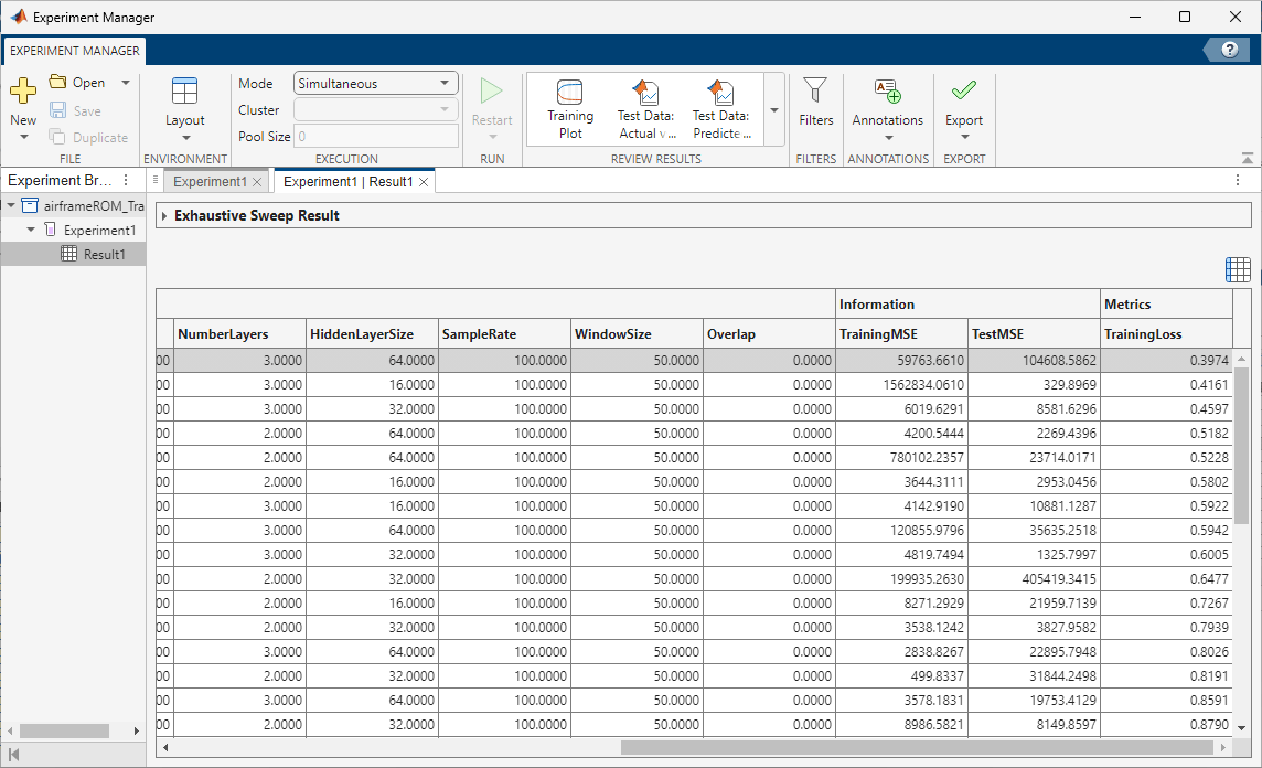
On the Experiment1 | Result1 tab, each row in the results table represents a trained model. The row for each model displays each of its hyperparameter values, as well as model performance information and metrics:

• TrainingMSE is the mean squared error calculated on the training data set. It is the average squared difference between the output obtained by simulating the original model and the output predicted by the trained model, using the training data values. Because the training data values were used to train the model, TrainingMSE shows how well the model fits the data used to train it.

• TestMSE is the mean squared error calculated on the test data set. It is the average squared difference between the output obtained by simulating the original model and the output predicted by the trained model, using the test data values. Because the test data values were not used to train the model, TestMSE shows how well the model performs on new data.

• TrainingLoss is the measure of inaccuracy of the model predictions calculated on the training data set. It shows how the model progresses by learning from the training data.

Sort the trained models by TrainingLoss in ascending order by clicking the arrow on the right of the TrainingLoss column header and selecting Sort in Ascending Order in the list that appears.

Of the models you trained, export the model with low TestMSE, reasonable TrainingMSE, and low TrainingLoss. When exporting the model, note down the values of its hyperparameters NumberInputLags and NumberOutputLags. To export a model as a workspace variable, first, select its row in the results table. On the Experiment Manager tab, in the Export menu, click Training Output. Name the workspace variable trainingOutput and click OK. Because the experiments that generate the training data use random pulse sequences for the input signal and Latin Hypercube sampling for the parameters, model performance might vary. To improve model performance, you can restrict the input and output lag hyperparameters to values that produced good fits, then rerun the training experiment.

For more information on hyperparameters and metrics, see Configure Options in Reduced Order Modeler (Simulink).

Use Trained NSS Model in Simulink

Note: You can begin at this step by loading a previously trained NSS model, trainedModelNSS.mat. This model was trained using data generated by experiments configured as shown in this example. To load the model, at the command line, enter:

load('trainedModelNSS.mat');

Warning: Updating objects saved with previous MATLAB version...
Resave your MAT files to improve loading speed.

Once you export a trained NSS model, you can use it in the airframeNSS Simulink model and compare its predictions to those of the original airframe model.

The trainingOutput variable stores the trained model and associated data.

trainingOutput

trainingOutput = struct with fields:
         NSSModel: [5×1 idNeuralStateSpace]
      TrainingMSE: 0.3394
          TestMSE: 0.3813
    Normalization: [1×1 struct]

To extract normalization, initial state, and output selection information, use the values of NumberInputLags and NumberOutputLags that you noted when exporting the model. The trained model trainedModelNSS.mat used 1 input lag and 0 output lags. This example uses these values.

nInLag = 1;
nOutLag = 0;

As part of model training, the NSS model normalizes the input and output signals. The airframeNSS model contains the Normalize and De-Normalize blocks that normalize the input to the trained models and denormalize their output, respectively. These blocks are configured to use normalization values that are assigned to specific workspace variables. Before you open and run the model, you must extract these values from the NSS training output and assign them to the correct variables.

trainingOutput.Normalization.Mu and trainingOutput.Normalization.Sigma store the normalization data for the input and output variables.

trainingOutput.Normalization.Mu

ans=1×6 table
     delta(t)     delta(t-1)    alpha(t)     ax(t)        q(t)        az(t) 
    __________    __________    _________    ______    __________    _______

    -0.0020418    -0.0020948    0.0048969    21.769    -0.0023691    -5.5468

trainingOutput.Normalization.Sigma

ans=1×6 table
    delta(t)    delta(t-1)    alpha(t)    ax(t)      q(t)      az(t) 
    ________    __________    ________    ______    _______    ______

    0.11519      0.11522      0.14162     3.6026    0.42278    168.77

Extract the input normalizations for delta and assign them to the variables specified in the Normalize block.

nMu = trainingOutput.Normalization.Mu{1,1};
nSigma = trainingOutput.Normalization.Sigma{1,1};

Extract the output normalizations for the output signals and any lagged inputs. Assign them to the variables specified in the De-Normalize block.

dnMu = trainingOutput.Normalization.Mu{1,1+nInLag+1:end}';
dnSigma = trainingOutput.Normalization.Sigma{1,1+nInLag+1:end}';
if nInLag > 0
    dnMu = [dnMu; ...
        trainingOutput.Normalization.Mu{1,2:(1+nInLag)}'];
    dnSigma = [dnSigma; ...
        trainingOutput.Normalization.Sigma{1,2:(1+nInLag)}'];
end

trainingOutput.NSSModel.StateName stores the states in the model.

trainingOutput.NSSModel.StateName

ans = 5×1 cell
    {'alpha(t)'  }
    {'ax(t)'     }
    {'q(t)'      }
    {'az(t)'     }
    {'delta(t-1)'}

Using the information about the order in which the states are stored, set the initial state for the NSS model. Normalize the initial state and assign it to the variable x0_nss specified in the Neural State Space Model block in the airframeNSS model.

x0_nss = [...
    0*ones(nOutLag+1,1); ...    %alpha
    35.7*ones(nOutLag+1,1); ... %ax
    0*ones(nOutLag+1,1); ...    %q     
    0*ones(nOutLag+1,1); ...    %az
    0*ones(nInLag,1)];          %delta(t-1)
x0_nss = (x0_nss-dnMu)./dnSigma;

The output of the NSS model is the augmented state vector which consists of the measured outputs (or states) followed by the lagged outputs (or lagged states). For this example, output only the lagged state by modifying the Selector block properties.

nOut = size(x0_nss,1); %All states
outIdx = 1 + (0:3)*(nOutLag+1); %Index into x(t) states

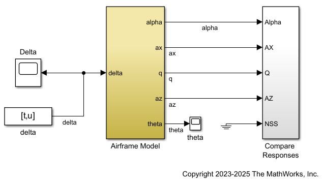
Open the airframeNSS model. This model includes the original airframe model and the blocks to implement the trained NSS model. You can verify that the Model parameter of the Neural State Space Model block is trainingOutput.NSSModel.

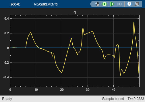
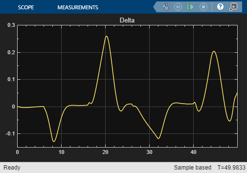
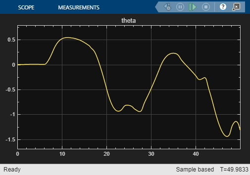
open_system("airframeNSS")

Run the airframeNSS model. The model scopes plot the output of both the original model and the NSS model.

sim("airframeNSS")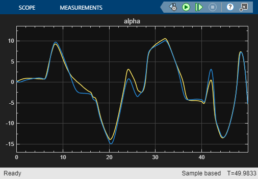

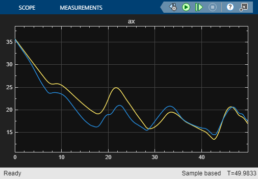
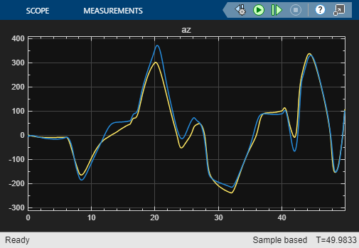
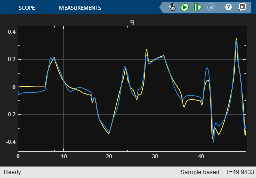
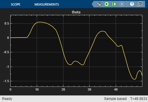
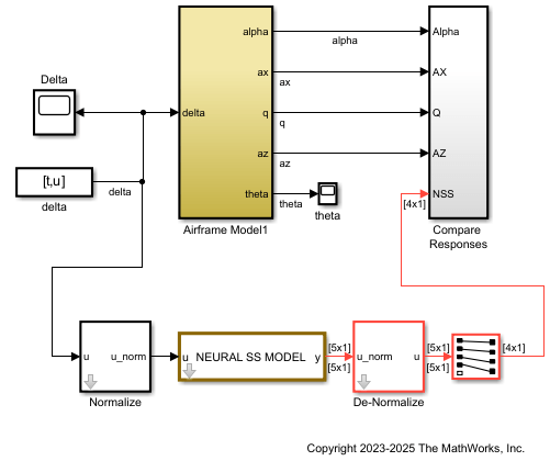
Note that you trained the NSS model using delta signals that were pulse sequences, but in this simulation, you use a realistic delta signal generated by a controller. The trained NSS model is able to generalize to this signal, thereby validating the model. To further improve the model, you can add experiments with same or different configuration settings in the Reduced Order Modeler app and use the data you collect to train new models.