Cylinder Design Parameter Sensitivity Analysis
This example shows how to perform a sensitivity analysis for tandem primary cylinder model in Simscape™. The example requires the Simulink® Design Optimization™ to be installed and licensed to run.
Introduction
Sensitivity Analysis: Sensitivity analysis can be used to study how the performance of a system depends on key design parameters. A few of the reasons to do this include:
To identify the design parameters that have significant impact on the model behavior.
To determine if the system displays the expected dependency on input parameters.
To determine permissible working range for key design parameters while still delivering the required system behavior and/or performance.
To identify if there are common sets of design parameters that influence system behavior in a similar way.
To determine requisite manufacturing tolerances to ensure system performance requirements are always met.
There are many approaches to sensitivity analysis including correlation and regression methods which are applied here to a tandem primary cylinder for use in automotive braking systems. In this example you will see functions from Sensitivity Analyzer app are used to perform this analysis.
Tandem Primary Cylinder: The tandem primary cylinder converts the applied mechanical force to the hydraulic force which is transferred to the wheels through the two pressure lines. For more information, see the Tandem Primary Cylinder example in MATLAB®.
Procedure for Sensitivity Analysis
Decide parameters for Sensitivity analysis: A change in a design parameter or application of a tolerance to a nominal design parameter value will affect the output of the system. There is a subset of parameters for which the output is more strongly dependent, and the first step is identify this subset via a sensitivity analysis.

For the sensitivity analysis we will consider following parameters:
Spring 1 stiffness coefficient. (tpcStiffness1Coeff)
Spring 2 stiffness coefficient. (tpcStiffness2Coeff)
Spring 1 initial deformation. (tpcSpring1Comp)
Spring 2 initial deformation. (tpcSpring2Comp)
Determine the range of the parameters: The variation in a property of an assembled part is a function of the manufacturing tolerances achieved. For example, the variation in the wire diameter of the spring will result in variation in the spring constant. For this example, we will assume 10% variation in the parameters listed above. It is assumed that the variation follows the uniform distribution.
We will be using Sensitivity Analyzer app to perform the sensitivity analysis.
Collect these param.Continuous object instances to a vector.
Sample the parameter space: In this section we generate 50 parameter combinations that span the parameter space. To generate the parameter combination instances the code below can be used. You can use higher number of samples for higher confidence.
You can observe the generated values using a scatter plot.

Define a system performance metric: The next step is to define requirements function that returns a metric of system performance. This metric can then be used to determine if the system is compliant with requirements, or not, for a given set of design parameter values. The pressure generated at Brake Pad 1 and Brake Pad 2 is a good metric for the efficacy of a tandem primary cylinder and hence these two signals are selected.
Next we create the experiment object and specify the input data.
Associate brake pressure 1 data with model output.
Associate brake pressure 2 data with model output.
Add brake pressure data to the sdo.experiment object.
Setup the Objective function: There are many options available in the Sensitivity Analyzer app depending on the objective of the analysis. Here a custom objective function is created. An alternative would be to use the Signal tracking objective from the app. The objective function compares the simulated output to the baseline provided to compute the cumulative error. In general, the objective function for the design parameter sensitivity analysis must be matched to a metric associated with the design functional requirement. Here the assumption is that the braking behavior using nominal design parameters is optimal, and the objective is to reduce variation from this behavior due to manufacturing tolerances in key design parameters.
Evaluate the experiment setup: Now that the setup is completed, you can evaluate the experiment.
Model evaluated at 50 samples.
Results from Simscape Example
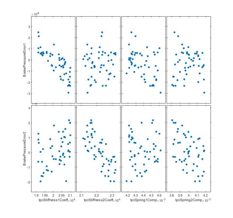
Plot the scatter plot of objectives versus each parameter under consideration.

Also, plot the sensitivity of each parameter using Ranked Standardized regression method.
                          BrakePressureError1    BrakePressureError2
                          ___________________    ___________________

    tpcStiffness1Coeff         -0.98197                0.022176
    tpcStiffness2Coeff         -0.21717                -0.94543
    tpcSpring1Comp             -0.44346               -0.051031
    tpcSpring2Comp             -0.16172                -0.62078
The higher value of sensitivity indicates that the design is dependent on the corresponding parameters and vice versa. A positive sign for the sensitivity indicates the objective function is directly proportional to the parameters under consideration whilst a negative sign indicates that the objective function is inversely proportional to the respective parameter.
From the table, we can infer that Port 1 brake pressure is highly dependent on Spring 1 stiffness and Spring 1 initial compression. This is expected because the pressure generated in Line 1 is directly associated with Spring 1. The stiffness and initial compression of Spring 2 also affects the error function by a small amount as it has comparatively low sensitivities. Similarly, Port 2 brake pressure is highly dependent on Spring 2 stiffness and Spring 2 initial compression and it is not affected by changes in Spring 1 stiffness and initial compression.
A Tornado plot gives a graphical representation of sensitivities of parameters for each objective function. In this case there are two objective functions, hence there are two subplots in the Tornado plot.
