Pattern Search Climbs Mount Washington
This example shows visually how pattern search optimizes a function. The function is the height of the terrain near Mount Washington, as a function of the x-y location. In order to find the top of Mount Washington, we minimize the objective function that is the negative of the height. (The Mount Washington in this example is the highest peak in the northeastern United States.)
The US Geological Survey provides data on the height of the terrain as a function of the x-y location on a grid. In order to be able to evaluate the height at an arbitrary point, the objective function interpolates the height from nearby grid points.
It would be faster, of course, to simply find the maximum value of the height as specified on the grid, using the max function. The point of this example is to show how the pattern search algorithm operates; it works on functions defined over continuous regions, not just grid points. Also, if it is computationally expensive to evaluate the objective function, then performing this evaluation on a complete grid, as required by the max function, will be much less efficient than using the pattern search algorithm, which samples a small subset of grid points.
How Pattern Search Works
Pattern search finds a local minimum of an objective function by the following method, called polling. In this description, words describing pattern search quantities are in bold. The search starts at an initial point, which is taken as the current point in the first step:
1. Generate a pattern of points, typically plus and minus the coordinate directions, times a mesh size, and center this pattern on the current point.
2. Evaluate the objective function at every point in the pattern.
3. If the minimum objective in the pattern is lower than the value at the current point, then the poll is successful, and the following happens:
3a. The minimum point found becomes the current point.
3b. The mesh size is doubled.
3c. The algorithm proceeds to Step 1.
4. If the poll is not successful, then the following happens:
4a. The mesh size is halved.
4b. If the mesh size is below a threshold, the iterations stop.
4c. Otherwise, the current point is retained, and the algorithm proceeds at Step 1.
This simple algorithm, with some minor modifications, provides a robust and straightforward method for optimization. It requires no gradients of the objective function. It lends itself to constraints, too, but this example and description deal only with unconstrained problems.
Preparing the Pattern Search
To prepare the pattern search, load the data in mtWashington.mat, which contains the USGS data on a 472-by-345 grid. The elevation, Z, is given in feet. The vectors x and y contain the base values of the grid spacing in the east and north directions respectively. The data file also contains the starting point for the search, X0.
load mtWashingtonThere are three MATLAB® files that perform the calculation of the objective function, and the plotting routines. They are:
1. terrainfun, which evaluates the negative of height at any x-y position. terrainfun uses the MATLAB function interp2 to perform two-dimensional linear interpolation. It takes the Z data and enables evaluation of the negative of the height at all x-y points.
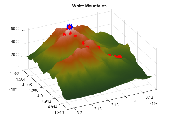
2. psoutputwashington, which draws a 3-d rendering of Mt. Washington. In addition, as the run progresses, it draws spheres around each point that is better (higher) than previously-visited points.
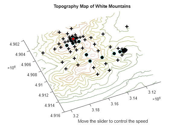
3. psplotwashington, which draws a contour map of Mt. Washington, and monitors a slider that controls the speed of the run. It shows where the pattern search algorithm looks for optima by drawing + signs at those points. It also draws spheres around each point that is better than previously-visited points.
In the example, patternsearch uses terrainfun as its objective function, psoutputwashington as an output function, and psplotwashington as a plot function. We prepare the functions to be passed to patternsearch in anonymous function syntax:
mtWashObjectiveFcn = @(xx) terrainfun(xx, x, y, Z);
mtWashOutputFcn    = @(xx,arg1,arg2) psoutputwashington(xx,arg1,arg2, x, y, Z);
mtWashPlotFcn      = @(xx,arg1) psplotwashington(xx,arg1, x, y, Z);
Pattern Search Options Settings
Next, we create options for pattern search. This set of options has the algorithm halt when the mesh size shrinks below 1, keeps the mesh unscaled (the same size in each direction), sets the initial mesh size to 10, and sets the output function and plot function:
options = optimoptions(@patternsearch,'MeshTolerance',1,'ScaleMesh',false, ...
    'InitialMeshSize',10,'UseCompletePoll',true,'PlotFcn',mtWashPlotFcn, ...
    'OutputFcn',mtWashOutputFcn,'UseVectorized',true);
Observing the Progress of Pattern Search
When you run this example you see two windows. One shows the points the pattern search algorithm chooses on a two-dimensional contour map of Mount Washington. This window has a slider that controls the delay between iterations of the algorithm (when it returns to Step 1 in the description of how pattern search works). Set the slider to a low position to speed the run, or to a high position to slow the run.
The other window shows a three-dimensional plot of Mount Washington, along with the steps the pattern search algorithm makes. You can rotate this plot while the run progresses to get different views.
[xfinal ffinal] = patternsearch(mtWashObjectiveFcn,X0,[],[],[],[],[], ...
    [],[],options)
patternsearch stopped because the mesh size was less than options.MeshTolerance.


xfinal = 1×2

      316130     4904295
ffinal =
-6280
The final point, xfinal, shows where the pattern search algorithm finished; this is the x-y location of the top of Mount Washington. The final objective function, ffinal, is the negative of the height of Mount Washington, 6280 feet. (This should be 6288 feet according to the Mount Washington Observatory).
Examine the files terrainfun.m, psoutputwashington.m, and psplotwashington.m to see how the interpolation and graphics work.
There are many options available for the pattern search algorithm. For example, the algorithm can take the first point it finds that is an improvement, rather than polling all the points in the pattern. It can poll the points in various orders. And it can use different patterns for the poll, both deterministic and random. Consult the Global Optimization Toolbox User's Guide for details.