Pareto Front for Two Objectives

Multiobjective Optimization with Two Objectives

This example shows how to find a Pareto set for a two-objective function of two variables. The example presents two approaches for minimizing: using the Optimize Live Editor task and working at the command line.

The two-objective function f(x), where x is also two-dimensional, is

$\begin{array}{l} f_{1} (x) = x_{1}^{4} + x_{2}^{4} + x_{1} x_{2} - (^{x_{1} x_{2}) 2} - 10 x_{1}^{2} \\ f_{2} (x) = x_{1}^{4} + x_{2}^{4} + x_{1} x_{2} - (^{x_{1} x_{2}) 2} . \end{array}$

Find Pareto Set Using Optimize Live Editor Task

Create a new live script by clicking the New Live Script button in the File section on the Home tab.
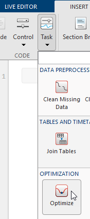
Insert an Optimize Live Editor task. Click the Insert tab and then, in the Code section, select Task > Optimize.
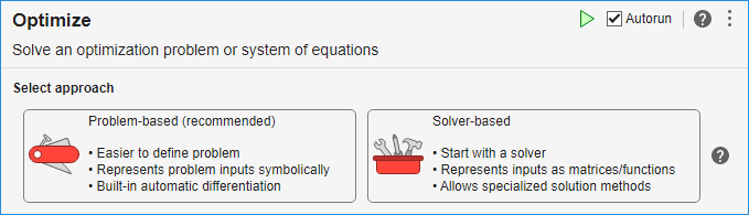
Click the Solver-based task.
For use in entering problem data, insert a new section by clicking the Section Break button on the Insert tab. New sections appear above and below the task.
In the new section above the task, enter the following code to define the number of variables and lower and upper bounds.
```
nvar = 2;
lb = [0 -5];
ub = [5 0];
```
To place these variables into the workspace, run the section by pressing Ctrl+Enter.
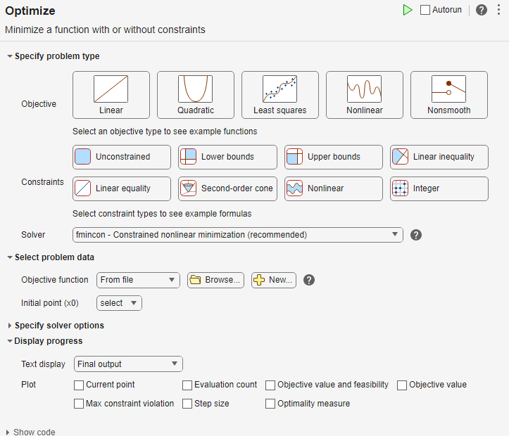
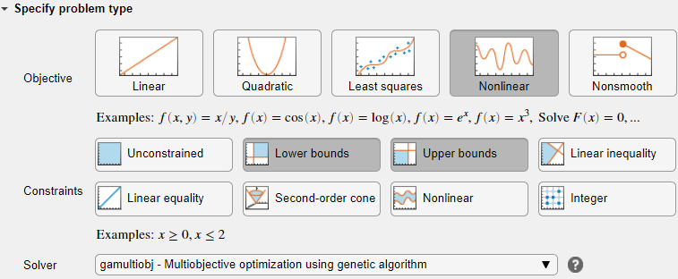
Specify Problem Type
In the Specify problem type section of the task, click the Objective > Nonlinear button.
Click the Constraints > Lower bounds and Upper bounds buttons.
Select Solver > gamultiobj - Multiobjective optimization using genetic algorithm.
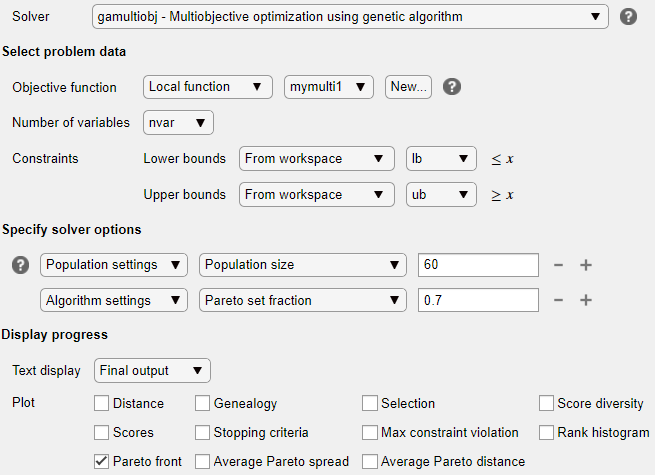
Select Problem Data
In the Select problem data section, select Objective function > Local function, and then click the New button. The function appears in a new section below the task.

Edit the resulting function definition to contain the following code.

function f = mymulti1(x)

f(2) = x(1)^4 + x(2)^4 + x(1)*x(2) - (x(1)*x(2))^2;
f(1) = f(2) - 10*x(1)^2;
end

In the Select problem data section, select the Local function > mymulti1 function.
Select Number of variables > nvar.
Select Lower bounds > From workspace > lb and Upper bounds > From workspace > ub.
Specify Solver Options
Expand the Specify solver options section of the task, and then click the Add button. To have a denser, more connected Pareto front, specify a larger-than-default populations by selecting Population settings > Population size > 60.
To have more of the population on the Pareto front than the default settings, click the + button. In the resulting options, select Algorithm > Pareto set fraction > 0.7.
Set Display Options
In the Display progress section of the task, select the Pareto front plot function.
Run Solver and Examine Results
To run the solver, click the options button ⁝ at the top right of the task window, and select Run Section. The plot appears in a separate figure window and in the task output area.
The plot shows the tradeoff between the two components of f, which is plotted in objective function space. For details, see the figure Figure 14-2, Set of Noninferior Solutions.

Find Pareto Set at the Command Line

To perform the same optimization at the command line, complete the following steps.

Create the mymulti1 objective function file on your MATLAB^® path.

function f = mymulti1(x)

f(2) = x(1)^4 + x(2)^4 + x(1)*x(2) - (x(1)*x(2))^2;
f(1) = f(2) - 10*x(1)^2;
end

Set the options and bounds.

options = optimoptions('gamultiobj','PopulationSize',60,...
          'ParetoFraction',0.7,'PlotFcn',@gaplotpareto);
lb = [0 -5];
ub = [5 0];

Run the optimization using the options.

[solution,ObjectiveValue] = gamultiobj(@mymulti1,2,...
                          [],[],[],[],lb,ub,options);

Both the Optimize Live Editor task and the command line allow you to formulate and solve problems, and they give identical results. The command line is more streamlined, but provides less help for choosing a solver, setting up the problem, and choosing options such as plot functions. You can also start a problem using Optimize, and then generate code for command line use, as in Constrained Nonlinear Problem Using Optimize Live Editor Task or Solver.

Alternate Views

You can view this problem in other ways. The following figure contains a plot of the level curves of the two objective functions, the Pareto frontier calculated by gamultiobj (boxes), and the x-values of the true Pareto frontier (diamonds connected by a nearly straight line). The true Pareto frontier points are where the level curves of the objective functions are parallel. The algorithm calculates these points by finding where the gradients of the objective functions are parallel. The figure is plotted in parameter space; see Figure 14-1, Mapping from Parameter Space into Objective Function Space.

Contours of objective functions, and Pareto frontier

gamultiobj finds the ends of the line segment, meaning it finds the full extent of the Pareto frontier.

Code for creating the figure

Create the solution data solution by running the optimization either in the Optimize Live Editor task or at the command line.

The Pareto frontier, the optimal tradeoff curve between the two objectives, is where the gradients of the two objective functions point in exactly opposite directions. The gradients are given in gg and gf in the following code:

function mout = mymulti2(x)
%
gg = [4*x(1)^3+x(2)-2*x(1)*(x(2)^2);
    x(1)+4*x(2)^3-2*(x(1)^2)*x(2)];
gf = gg - [20*x(1);0];

mout = gf(1)*gg(2) - gf(2)*gg(1);

mout = 0 if the two gradients are parallel.

This code creates the plot.

[x,y] = meshgrid(0:.01:3,-2:.01:0);
[myf,myg] = mymulti(x,y);
mygg = sqrt(myg+.26); % This spaces the contours better
myff = sqrt(myf+40); % This spaces the contours better
a = [.7,fzero(@(t)mymulti2([.7,t]),[-2;0])];
% fzero calculates where mout = 0
for jj = 0.8:0.1:2.6
    a = [a;[jj,fzero(@(t)mymulti2([jj,t]),[-2;0])]];
end
a = [a;[2.65,fzero(@(t)mymulti2([2.65,t]),[-2;0])]];
figure
hold on
contour(x,y,mygg,50)
contour(x,y,myff,50)
gam = plot(solution(:,1),solution(:,2),'ks');
tru = plot(a(:,1),a(:,2),'-dr');
legend([gam tru],'Points calculated by \bf{\fontname{Courier}gamultiobj}',...
    'True Pareto frontier')
hold off

The function mymulti(x,y) is a vectorized version of the multiobjective fitness function.

function [f,g] = mymulti(x,y)
%
g = x.^4 + y.^4 + x.*y - (x.^2).*(y.^2);
f = g - 10*x.^2;
end