Constrained Minimization Using patternsearch and Optimize Live Editor Task

This example shows how to solve a constrained minimization problem using both the Optimize Live Editor task, which offers a visual approach, and the command line.

Problem Description

The problem involves using linear and nonlinear constraints when minimizing a nonlinear function with patternsearch. The objective function is

$$F(x)=\frac{1}{2}{x}^{T}Hx+f^{T}x,$$

where

H = [36 17 19 12  8 15; 
     17 33 18 11  7 14; 
     19 18 43 13  8 16;
     12 11 13 18  6 11; 
      8  7  8  6  9  8; 
     15 14 16 11  8 29];

f = [ 20 15 21 18 29 24 ]';
 
F = @(x)0.5*x'*H*x + f'*x;

The linear constraints are

$$\begin{array}{c}A\cdot x\le b,\\ Aeq\cdot x=beq,\end{array}$$

where

A = [-8 7 3 -4 9 0];
b = 7;
Aeq = [7 1 8 3 3 3;
      5 0 -5 1 -5 8;
     -2 -6 7 1 1 9;
      1 -1 2 -2 3 -3];
beq = [84 62 65 1]';

Enter the preceding code sections to get the problem variables into your workspace before proceeding.

Solve Using patternsearch in Optimize Live Editor Task

1. Create a new live script by clicking the New Live Script button in the File section on the Home tab.

   

2. Insert an Optimize Live Editor task. Click the Insert tab and then, in the Code section, select Task > Optimize.

   

   

3. For this example, choose the solver-based task.

   

4. Specify Problem Type

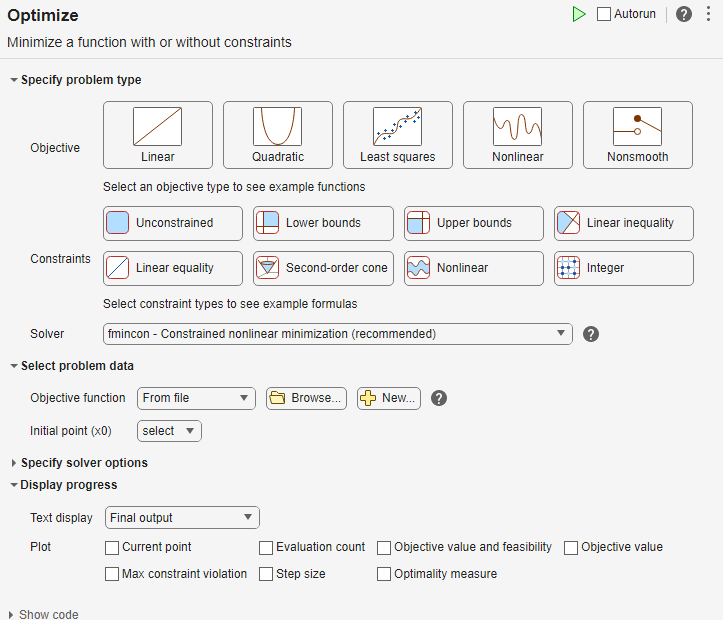
   In the Specify problem type section of the task, click the Objective > Nonlinear button.

5. Click the Constraints > Linear inequality and Linear equality buttons.

6. Select Solver > patternsearch - Pattern search.

7. Select Problem Data

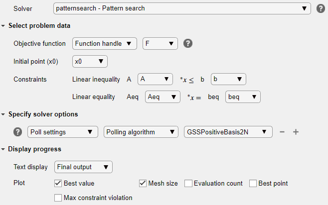
   Enter the problem variables in the Select problem data section of the task. To specify the objective function, select Objective function > Function handle and choose F.

8. Set the inequality constraints to A and b. Set the equality constraints to Aeq and beq.

9. To set the initial point, you first need to create a new section above the task. To do so, click the Section Break button on the Insert tab. In the new section above the task, enter the following code for the initial point.

   x0 = [2 1 0 9 1 0]';

10. Run the section to place x0 into the workspace. To run the section, place the cursor in the section and press Ctrl+Enter or click the blue striped bar to the left of the line number.

11. In the Select problem data section of the task, set x0 as the initial point.

12. Specify Solver Options

    Because this problem is linearly constrained, specify an additional solver option. Expand the Specify solver options section of the task, and then click the Add button. Set the Poll settings > Poll method to GSSPositiveBasis2N. For more information about the efficiency of the GSS poll methods for linearly constrained problems, see Compare the Efficiency of Poll Options.

13. Set Display Options

    In the Display progress section of the task, select the Best value and Mesh size plot functions.

    Your setup looks like this:

    

14. Run Solver and Examine Results

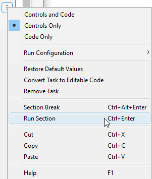
    To run the solver, click the options button ⁝ at the top right of the task window, and select Run Section.

    

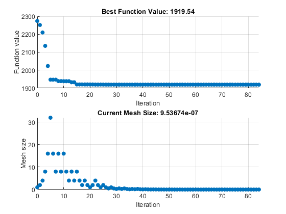
    The plots appear in a separate figure window and in the task output area.

    

15. To obtain the solution point and objective function value at the solution, look at the top of the task.

    

    The Optimize Live Editor task returns the solution in a variable named solution and returns the objective function value in a variable named objectiveValue. View these values by entering the following code in the section below the task and then running the section, or by entering the code at the MATLAB^® command line.

    disp(solution)

        8.5165
       -6.1094
        4.0989
        1.2877
       -4.2348
        2.1812

    disp(objectiveValue)

       1.9195e+03

16. Include Nonlinear Constraints

    Add the following nonlinear constraints to the problem.

    $$\begin{array}{c}-1.5+x_1{x}_2+x_1-x_2\le 0\\ -x_1{x}_2-10\le 0.\end{array}$$

    To include these constraints, first click the Constraints > Nonlinear button.

    

17. In the Select problem data section, under Constraints, select Nonlinear > Local function and then click the New button. The function appears in a new section below the task. Edit the resulting code to contain the following lines.

    function [c, ceq] = double_ineq(x)
    c = [-1.5 + x(1)*x(2) + x(1) - x(2);
        -x(1)*x(2) - 10];
    ceq = [];
    end

18. In the Nonlinear constraints section, select double_ineq.

19. The nonlinear constraint algorithm causes patternsearch to take many function evaluations. In the Specify solver options section, click the plus sign to the right of the current options to display additional options. Then increase the maximum function evaluation limit to 5e4.

    

20. Run the task again to rerun the optimization.

    

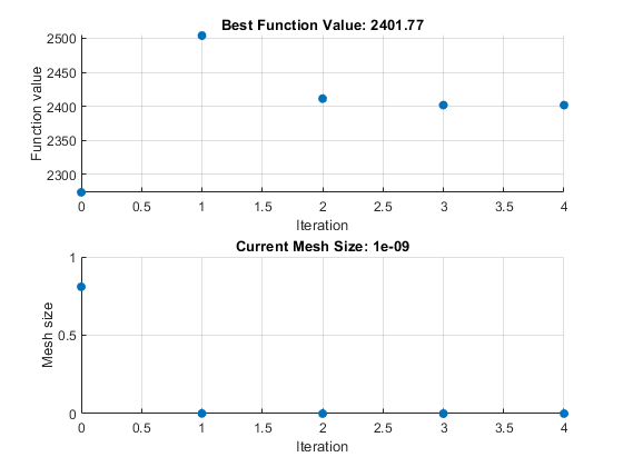
21. View the solution and objective function value.

    disp(solution)

        7.2083
       -1.3873
        4.9579
       -3.1393
       -3.1843
        4.7457

    disp(objectiveValue)

       2.4018e+03

The objective function value is higher than the value in the problem without nonlinear constraints. The previous solution is not feasible with respect to the nonlinear constraints.

The plots show many fewer iterations than before because the nonlinear constraint algorithm changes the patternsearch algorithm to include another outer loop to solve a modified problem. The outer loop reduces the modification to the problem at each major iteration. In this case, the algorithm makes only four outer iterations. For algorithm details, see Nonlinear Constraint Solver Algorithm for Pattern Search.

Solve Using patternsearch at the Command Line

To solve the original problem (only linear constraints) at the command line, execute the following code.

x0 = [2 1 0 9 1 0]';
options = optimoptions('patternsearch',...
    'PollMethod','GSSPositiveBasis2N',...
    'PlotFcn',{'psplotbestf','psplotmeshsize'});
lb = [];
ub = [];
nonlcon = [];
[x,fval] = patternsearch(F,x0,A,b,Aeq,beq,lb,ub,nonlcon,options)

Optimization terminated: mesh size less than options.MeshTolerance.

x =

    8.5165
   -6.1094
    4.0989
    1.2877
   -4.2348
    2.1812


fval =

   1.9195e+03

patternsearch generates the first pair of plots shown in the Optimize Live Editor task example.

To include the nonlinear constraints, save the following code to a file named double_ineq.m on the MATLAB path.

function [c, ceq] = double_ineq(x)
c = [-1.5 + x(1)*x(2) + x(1) - x(2);
    -x(1)*x(2) - 10];
ceq = [];
end

To allow the solver to run to completion with nonlinear constraints, increase the allowed number of function evaluations.

options.MaxFunctionEvaluations = 5e4;

Solve the problem including nonlinear constraints.

nonlcon = @double_ineq;
[x,fval] = patternsearch(F,x0,A,b,Aeq,beq,lb,ub,nonlcon,options)

Optimization terminated: mesh size less than options.MeshTolerance
 and constraint violation is less than options.ConstraintTolerance.

x =

    7.2083
   -1.3873
    4.9579
   -3.1393
   -3.1843
    4.7457


fval =

   2.4018e+03

patternsearch also generates the second pair of plots shown in the Optimize Live Editor task example.

Both the Optimize Live Editor task and the command line allow you to formulate and solve problems, and they give identical results. The command line is more streamlined, but provides less help for choosing a solver, setting up the problem, and choosing options such as plot functions. You can also start a problem using Optimize, and then generate code for command line use, as in Constrained Nonlinear Problem Using Optimize Live Editor Task or Solver.