AHRS

Orientation from accelerometer, gyroscope, and magnetometer readings

Since R2020a

• 

×

Libraries:
Navigation Toolbox / Multisensor Positioning / Navigation Filters
Sensor Fusion and Tracking Toolbox / Multisensor Positioning / Navigation Filters

Description

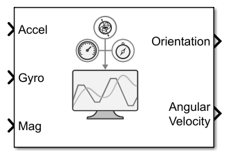
The AHRS Simulink^® block fuses accelerometer, magnetometer, and gyroscope sensor data to estimate device orientation.

Examples

IMU Sensor Fusion with Simulink

Generate and fuse IMU sensor data using Simulink®. You can accurately model the behavior of an accelerometer, a gyroscope, and a magnetometer and fuse their outputs to compute orientation.

• Open Script

Ports

Input

Accel — Accelerometer readings in sensor body coordinate system (m/s²)

N-by-3 matrix of real scalar

Accelerometer readings in the sensor body coordinate system in m/s², specified as an N-by-3 matrix of real scalars. N is the number of samples, and the three columns of Accel represent the [x y z] measurements, respectively.

Data Types: single | double

Gyro — Gyroscope readings in sensor body coordinate system (rad/s)

N-by-3 matrix of real scalar

Gyroscope readings in the sensor body coordinate system in rad/s, specified as an N-by-3 matrix of real scalars. N is the number of samples, and the three columns of Gyro represent the [x y z] measurements, respectively.

Data Types: single | double

Mag — Magnetometer readings in sensor body coordinate system (µT)

N-by-3 matrix of real scalar

Magnetometer readings in the sensor body coordinate system in µT, specified as an N-by-3 matrix of real scalars. N is the number of samples, and the three columns of magReadings represent the [x y z] measurements, respectively.

Data Types: single | double

Output

Orientation — Orientation of sensor body frame relative to navigation frame

M-by-4 array of scalar | 3-by-3-by-M-element rotation matrix

Orientation of the sensor body frame relative to the navigation frame, return as an M-by-4 array of scalars or a 3-by-3-by-M array of rotation matrices. Each row the of the N-by-4 array is assumed to be the four elements of a quaternion. The number of input samples, N, and the Decimation Factor parameter determine the output size M.

Data Types: single | double

Angular Velocity — Angular velocity in sensor body coordinate system (rad/s)

M-by-3 array of real scalar (default)

Angular velocity with gyroscope bias removed in the sensor body coordinate system in rad/s, returned as an M-by-3 array of real scalars. The number of input samples, N, and the Decimation Factor parameter determine the output size M.

Data Types: single | double

Parameters

Main

Reference frame — Navigation reference frame

NED (default) | ENU

Navigation reference frame, specified as NED (North-East-Down) or ENU (East-North-Up).

Decimation factor — Decimation factor

1 (default) | positive integer

Decimation factor by which to reduce the input sensor data rate, specified as a positive integer.

The number of rows of the inputs –– Accel, Gyro , and Mag –– must be a multiple of the decimation factor.

Data Types: single | double

Initial process noise — Initial process noise

ahrsfilter.defaultProcessNoise (default) | 12-by-12 matrix of real scalar

Initial process noise, specified as a 12-by-12 matrix of real scalars. The default value, ahrsfilter.defaultProcessNoise, is a 12-by-12 diagonal matrix as:

  Columns 1 through 6

   0.000006092348396                   0                   0                   0                   0                   0
                   0   0.000006092348396                   0                   0                   0                   0
                   0                   0   0.000006092348396                   0                   0                   0
                   0                   0                   0   0.000076154354947                   0                   0
                   0                   0                   0                   0   0.000076154354947                   0
                   0                   0                   0                   0                   0   0.000076154354947
                   0                   0                   0                   0                   0                   0
                   0                   0                   0                   0                   0                   0
                   0                   0                   0                   0                   0                   0
                   0                   0                   0                   0                   0                   0
                   0                   0                   0                   0                   0                   0
                   0                   0                   0                   0                   0                   0

  Columns 7 through 12

                   0                   0                   0                   0                   0                   0
                   0                   0                   0                   0                   0                   0
                   0                   0                   0                   0                   0                   0
                   0                   0                   0                   0                   0                   0
                   0                   0                   0                   0                   0                   0
                   0                   0                   0                   0                   0                   0
   0.009623610000000                   0                   0                   0                   0                   0
                   0   0.009623610000000                   0                   0                   0                   0
                   0                   0   0.009623610000000                   0                   0                   0
                   0                   0                   0   0.600000000000000                   0                   0
                   0                   0                   0                   0   0.600000000000000                   0
                   0                   0                   0                   0                   0   0.600000000000000

Data Types: single | double

Orientation format — Orientation output format

'quaternion' (default) | 'Rotation matrix'

Output orientation format, specified as 'quaternion' or 'Rotation matrix':

• 'quaternion' –– Output is an M-by-4 array of real scalars. Each row of the array represents the four components of a quaternion.

• 'Rotation matrix' –– Output is a 3-by-3-by-M rotation matrix.

The output size M depends on the input dimension N and the Decimation Factor parameter.

Data Types: char | string

Simulate using — Type of simulation to run

Interpreted Execution (default) | Code Generation

• Interpreted execution — Simulate the model using the MATLAB^® interpreter. This option shortens startup time. In Interpreted execution mode, you can debug the source code of the block.

• Code generation — Simulate the model using generated C code. The first time you run a simulation, Simulink generates C code for the block. The C code is reused for subsequent simulations as long as the model does not change. This option requires additional startup time.

Measurement Noise

Accelerometer noise ((m/s²)²) — Variance of accelerometer signal noise ((m/s²)²)

0.0001924722 (default) | positive real scalar

Variance of accelerometer signal noise in (m/s²)², specified as a positive real scalar.

Data Types: single | double

Gyroscope noise ((rad/s)²) — Variance of gyroscope signal noise ((rad/s)²)

9.1385e-5 (default) | positive real scalar

Variance of gyroscope signal noise in (rad/s)², specified as a positive real scalar.

Data Types: single | double

Magnetometer noise (μT²) — Variance of magnetometer signal noise (μT²)

0.1 (default) | positive real scalar

Variance of magnetometer signal noise in μT², specified as a positive real scalar.

Data Types: single | double

Gyroscope drift noise (rad/s) — Variance of gyroscope offset drift ((rad/s)²)

3.0462e-13 (default) | positive real scalar

Variance of gyroscope offset drift in (rad/s)², specified as a positive real scalar.

Data Types: single | double

Environmental Noise

Linear acceleration noise ((m/s²)²) — Variance of linear acceleration noise (m/s²)²

0.0096236100000000012 (default) | positive real scalar

Variance of linear acceleration noise in (m/s²)², specified as a positive real scalar. Linear acceleration is modeled as a lowpass-filtered white noise process.

Data Types: single | double

Magnetic disturbance noise (μT²) — Variance of magnetic disturbance noise ((μT)²)

0.5 (default) | real finite positive scalar

Variance of magnetic disturbance noise in μT², specified as a real finite positive scalar.

Data Types: single | double

Linear acceleration decay factor — Decay factor for linear acceleration drift

0.5 (default) | scalar in the range [0,1)

Decay factor for linear acceleration drift, specified as a scalar in the range [0,1). If linear acceleration changes quickly, set this parameter to a lower value. If linear acceleration changes slowly, set this parameter to a higher value. Linear acceleration drift is modeled as a lowpass-filtered white noise process.

Data Types: single | double

Magnetic disturbance decay factor — Decay factor for magnetic disturbance

0.5 (default) | positive scalar in the range [0,1]

Decay factor for magnetic disturbance, specified as a positive scalar in the range [0,1]. Magnetic disturbance is modeled as a first order Markov process.

Data Types: single | double

Magnetic field strength (μT) — Magnetic field strength (μT)

50 (default) | real positive scalar

Magnetic field strength in μT, specified as a real positive scalar. The magnetic field strength is an estimate of the magnetic field strength of the Earth at the current location.

Data Types: single | double

Algorithms

Note: The following algorithm only applies to an NED reference frame.

The AHRS block uses the nine-axis Kalman filter structure described in [1]. The algorithm attempts to track the errors in orientation, gyroscope offset, linear acceleration, and magnetic disturbance to output the final orientation and angular velocity. Instead of tracking the orientation directly, the indirect Kalman filter models the error process, x, with a recursive update:

$$x_k=\left[\begin{array}{c}{\theta }_k\\ b_k\\ a_k\\ d_k\end{array}\right]=F_k\left[\begin{array}{c}{\theta }_{k-1}\\ b_{k-1}\\ a_{k-1}\\ d_{k-1}\end{array}\right]+w_k$$

where x_k is a 12-by-1 vector consisting of:

• θ_k –– 3-by-1 orientation error vector, in degrees, at time k

• b_k –– 3-by-1 gyroscope zero angular rate bias vector, in deg/s, at time k

• a_k –– 3-by-1 acceleration error vector measured in the sensor frame, in g, at time k

• d_k –– 3-by-1 magnetic disturbance error vector measured in the sensor frame, in µT, at time k

and where w_k is a 12-by-1 additive noise vector, and F_k is the state transition model.

Because x_k is defined as the error process, the a priori estimate is always zero, and therefore the state transition model, F_k, is zero. This insight results in the following reduction of the standard Kalman equations:

Standard Kalman equations:

$$\begin{array}{l}{x}_k^{-}=F_k{x}_{k-1}^{+}\\ P_k^{-}=F_k{P}_{k-1}^{+}{F}_k^T+Q_k\\ \\ y_k=z_k-H_k{x}_k^{-}\\ S_k=R_k+H_k{P}_k^{-}{H}_k{}^T\\ K_k=P_k^{-}{H}_k^T{\left(S_k\right)}^{-1}\\ x_k^{+}=x_k^{-}+K_k{y}_k\\ P_k^{+}=P_k{}^{-}-K_k{H}_k{P}_k^{-}\end{array}$$

Kalman equations used in this algorithm:

$$\begin{array}{l}{x}_k^{-}=0\\ P_k^{-}=Q_k\\ \\ y_k=z_k\\ S_k=R_k+H_k{P}_k^{-}{H}_k{}^T\\ K_k=P_k^{-}{H}_k^T{\left(S_k\right)}^{-1}\\ x_k^{+}=K_k{y}_k\\ P_k^{+}=P_k{}^{-}-K_k{H}_k{P}_k^{-}\end{array}$$

where:

• x_k⁻ –– predicted (a priori) state estimate; the error process

• P_k⁻ –– predicted (a priori) estimate covariance

• y_k –– innovation

• S_k –– innovation covariance

• K_k –– Kalman gain

• x_k⁺ –– updated (a posteriori) state estimate

• P_k⁺ –– updated (a posteriori) estimate covariance

k represents the iteration, the superscript ⁺ represents an a posteriori estimate, and the superscript ⁻ represents an a priori estimate.

The graphic and following steps describe a single frame-based iteration through the algorithm.

Before the first iteration, the accelReadings, gyroReadings, and magReadings inputs are chunked into DecimationFactor-by-3 frames. For each chunk, the algorithm uses the most current accelerometer and magnetometer readings corresponding to the chunk of gyroscope readings.

Detailed Overview

Walk through the algorithm for an explanation of each stage of the detailed overview.

Model

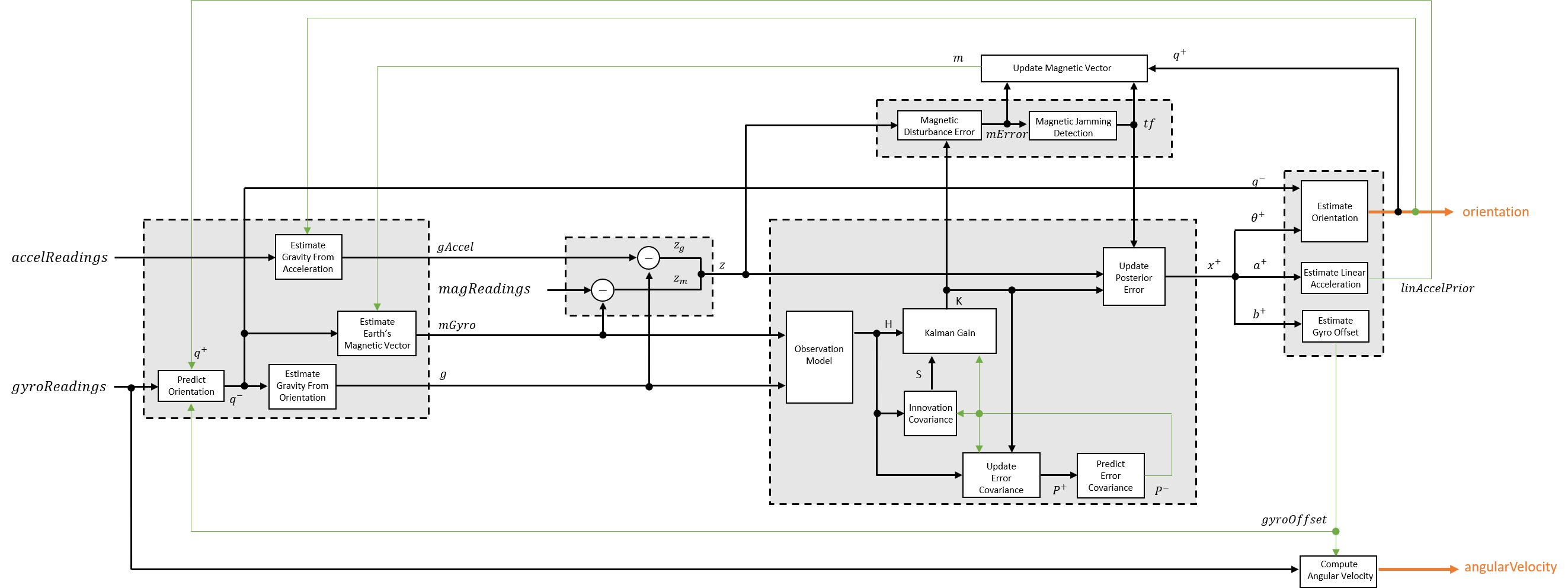
The algorithm models acceleration and angular change as linear processes.

Predict Orientation

The orientation for the current frame is predicted by first estimating the angular change from the previous frame:

$$\Delta {\phi }_{N\times 3}=\frac{\left(gyroReading{s}_{N\times 3}-gyroOffse{t}_{1\times 3}\right)}{fs}$$

where N is the decimation factor specified by the Decimation factor and fs is the sample rate.

The angular change is converted into quaternions using the rotvec quaternion construction syntax:

$$\Delta Q_{N\times 1}=\mathrm{quaternion}(\Delta {\phi }_{N\times 3},\text{'}rotvec\text{'})$$

The previous orientation estimate is updated by rotating it by ΔQ:

$$q_{1\times 1}^{-}=\left(q_{1\times 1}^{+}\right)\left({\displaystyle \prod _{n=1}^N\Delta Q_n}\right)$$

During the first iteration, the orientation estimate, q⁻, is initialized by ecompass.

Estimate Gravity from Orientation

The gravity vector is interpreted as the third column of the quaternion, q⁻, in rotation matrix form:

$$g_{1\times 3}={\left(rPrior(:,3)\right)}^T$$

Estimate Gravity from Acceleration

A second gravity vector estimation is made by subtracting the decayed linear acceleration estimate of the previous iteration from the accelerometer readings:

$$gAcce{l}_{1\times 3}=accelReading{s}_{1\times 3}-linAccelprio{r}_{1\times 3}$$

Estimate Earth's Magnetic Vector

Earth's magnetic vector is estimated by rotating the magnetic vector estimate from the previous iteration by the a priori orientation estimate, in rotation matrix form:

$$mGyr{o}_{1\times 3}={\left(\left(rPrior\right)\left(m^T\right)\right)}^T$$

Error Model

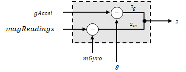
The error model combines two differences:

• The difference between the gravity estimate from the accelerometer readings and the gravity estimate from the gyroscope readings: $$z_g=g-gAccel$$

• The difference between the magnetic vector estimate from the gyroscope readings and the magnetic vector estimate from the magnetometer:$$z_m=mGyro-magReadings$$

Magnetometer Correct

The magnetometer correct estimates the error in the magnetic vector estimate and detects magnetic jamming.

Magnetometer Disturbance Error

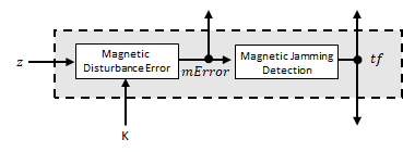
The magnetic disturbance error is calculated by matrix multiplication of the Kalman gain associated with the magnetic vector with the error signal:

$$mErro{r}_{3\times 1}={\left(\left(K{(\text{10:12},:)}_{3\times 6}\right){\left(z_{1\times 6}\right)}^T\right)}^T$$

The Kalman gain, K, is the Kalman gain calculated in the current iteration.

Magnetic Jamming Detection

Magnetic jamming is determined by verifying that the power of the detected magnetic disturbance is less than or equal to four times the power of the expected magnetic field strength:

$$tf=\{\begin{array}{c}\text{true}\\ \text{false}\end{array}\begin{array}{c}\text{if}\\ \text{else}\end{array}\begin{array}{c}{{\displaystyle \sum \left|mError\right|}}^2>\left(4\right){\left(\text{ExpectedMagneticFieldStrength}\right)}^2\\ \end{array}$$

ExpectedMagneticFieldStrength is a property of ahrsfilter.

Kalman Equations

The Kalman equations use the gravity estimate derived from the gyroscope readings, g, the magnetic vector estimate derived from the gyroscope readings, mGyro, and the observation of the error process, z, to update the Kalman gain and intermediary covariance matrices. The Kalman gain is applied to the error signal, z, to output an a posteriori error estimate, x⁺.

Observation Model

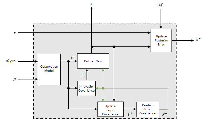
The observation model maps the 1-by-3 observed states, g and mGyro, into the 6-by-12 true state, H.

The observation model is constructed as:

$$H_{3\times 9}=\left[\begin{array}{cccccccccccc}0& g_z& -g_y& 0& -\kappa g_z& \kappa g_y& 1& 0& 0& 0& 0& 0\\ -g_z& 0& g_x& \kappa g_z& 0& -\kappa g_x& 0& 1& 0& 0& 0& 0\\ g_y& -g_x& 0& -\kappa g_y& \kappa g_x& 0& 0& 0& 1& 0& 0& 0\\ 0& m_z& -m_y& 0& -\kappa m_z& -\kappa m_y& 0& 0& 0& -1& 0& 0\\ -m_z& 0& m_x& \kappa m_z& 0& -\kappa m_x& 0& 0& 0& 0& -1& 0\\ m_y& -m_x& 0& -\kappa m_y& \kappa m_x& 0& 0& 0& 0& 0& 0& -1\end{array}\right]$$

where g_x, g_y, and g_z are the x-, y-, and z-elements of the gravity vector estimated from the a priori orientation, respectively. m_x, m_y, and m_z are the x-, y-, and z-elements of the magnetic vector estimated from the a priori orientation, respectively. κ is a constant determined by the Sample rate and Decimation factor properties: κ = Decimation factor/Sample rate.

Innovation Covariance

The innovation covariance is a 6-by-6 matrix used to track the variability in the measurements. The innovation covariance matrix is calculated as:

$$S_{6x6}=R_{6x6}+\left(H_{6x12}\right)\left(P_{{}_{12x12}}^{-}\right){\left(H_{6x12}\right)}^T$$

where

• H is the observation model matrix

• P⁻ is the predicted (a priori) estimate of the covariance of the observation model calculated in the previous iteration

• R is the covariance of the observation model noise, calculated as:

  $$R_{6\times 6}=\left[\begin{array}{cccccc}acce{l}_{\text{noise}}& 0& 0& 0& 0& 0\\ 0& acce{l}_{\text{noise}}& 0& 0& 0& 0\\ 0& 0& acce{l}_{\text{noise}}& 0& 0& 0\\ 0& 0& 0& ma{g}_{\text{noise}}& 0& 0\\ 0& 0& 0& 0& ma{g}_{\text{noise}}& 0\\ 0& 0& 0& 0& 0& ma{g}_{\text{noise}}\end{array}\right]$$

  where

  $$acce{l}_{\text{noise}}=\text{AccelerometerNoise}\text{+}\text{LinearAccelerationNoise}\text{+}{\kappa }^2\left(\text{GyroscopeDriftNoise}\text{+}\text{GyroscopeNoise}\right)$$

  and

  $$ma{g}_{\text{noise}}=\text{MagnetometerNoise}\text{+}\text{MagneticDisturbanceNoise}\text{+}{\kappa }^2\left(\text{GyroscopeDriftNoise}\text{+}\text{GyroscopeNoise}\right)$$

Update Error Estimate Covariance

The error estimate covariance is a 12-by-12 matrix used to track the variability in the state.

The error estimate covariance matrix is updated as:

$$P_{{}_{12\times 12}}^{+}=P_{{}_{12\times 12}}^{-}-\left(K_{12\times 6}\right)\left(H_{6\times 12}\right)\left(P_{{}_{12\times 12}}^{-}\right)$$

where K is the Kalman gain, H is the measurement matrix, and P⁻ is the error estimate covariance calculated during the previous iteration.

Predict Error Estimate Covariance

The error estimate covariance is a 12-by-12 matrix used to track the variability in the state. The a priori error estimate covariance, P⁻, is set to the process noise covariance, Q, determined during the previous iteration. Q is calculated as a function of the a posteriori error estimate covariance, P⁺. When calculating Q, it is assumed that the cross-correlation terms are negligible compared to the autocorrelation terms, and are set to zero:

$$Q=\left[\begin{array}{cccccccccccc}{P}^{+}(1)+{\kappa }^2\left(P^{+}(40)+\beta +\eta \right)& 0& 0& -\kappa \left(P^{+}(40)+\beta \right)& 0& 0& 0& 0& 0& 0& 0& 0\\ 0& P^{+}(14)+{\kappa }^2\left(P^{+}(53)+\beta +\eta \right)& 0& 0& -\kappa \left(P^{+}(53)+\beta \right)& 0& 0& 0& 0& 0& 0& 0\\ 0& 0& P^{+}(27)+{\kappa }^2\left(P^{+}(66)+\beta +\eta \right)& 0& 0& -\kappa \left(P^{+}(66)+\beta \right)& 0& 0& 0& 0& 0& 0\\ -\kappa \left(P^{+}(40)+\beta \right)& 0& 0& P^{+}(40)+\beta & 0& 0& 0& 0& 0& 0& 0& 0\\ 0& -\kappa \left(P^{+}(53)+\beta \right)& 0& 0& P^{+}(53)+\beta & 0& 0& 0& 0& 0& 0& 0\\ 0& 0& -\kappa \left(P^{+}(66)+\beta \right)& 0& 0& P^{+}(66)+\beta & 0& 0& 0& 0& 0& 0\\ 0& 0& 0& 0& 0& 0& {\nu }^2{P}^{+}(79)+\xi & 0& 0& 0& 0& 0\\ 0& 0& 0& 0& 0& 0& 0& {\nu }^2{P}^{+}(92)+\xi & 0& 0& 0& 0\\ 0& 0& 0& 0& 0& 0& 0& 0& {\nu }^2{P}^{+}(105)+\xi & 0& 0& 0\\ 0& 0& 0& 0& 0& 0& 0& 0& 0& {\sigma }^2{P}^{+}(118)+\gamma & 0& 0\\ 0& 0& 0& 0& 0& 0& 0& 0& 0& 0& {\sigma }^2{P}^{+}(131)+\gamma & 0\\ 0& 0& 0& 0& 0& 0& 0& 0& 0& 0& 0& {\sigma }^2{P}^{+}(144)+\gamma \end{array}\right]$$

where

• P⁺ –– is the updated (a posteriori) error estimate covariance

• κ –– Decimation factor divided by sample rate.

• β –– Gyroscope drift noise.

• η –– Gyroscope noise.

• ν –– Linear acceleration decay factor.

• ξ –– Linear acceleration noise.

• σ –– Magnetic disturbance decay factor.

• γ –– Magnetic disturbance noise.

Kalman Gain

The Kalman gain matrix is a 12-by-6 matrix used to weight the innovation. In this algorithm, the innovation is interpreted as the error process, z.

The Kalman gain matrix is constructed as:

$$K_{12\times 6}=\left(P_{{}_{12\times 12}}^{-}\right){\left(H_{6\times 12}\right)}^T{\left({\left(S_{6\times 6}\right)}^T\right)}^{-1}$$

where

• P⁻ –– predicted error covariance

• H –– observation model

• S –– innovation covariance

Update a Posteriori Error

The a posterior error estimate is determined by combining the Kalman gain matrix with the error in the gravity vector and magnetic vector estimations:

$$x_{12\times 1}=\left(K_{12\times 6}\right){(z_{1\times 6})}^T$$

If magnetic jamming is detected in the current iteration, the magnetic vector error signal is ignored, and the a posterior error estimate is calculated as:

$$x_{9\times 1}=\left(K(\text{1:9},\text{1:3}\right){(z_g)}^T$$

Correct

Estimate Orientation

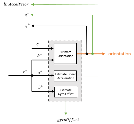
The orientation estimate is updated by multiplying the previous estimation by the error:

$$q^{+}=\left(q^{-}\right)\left({\theta }^{+}\right)$$

Estimate Linear Acceleration

The linear acceleration estimation is updated by decaying the linear acceleration estimation from the previous iteration and subtracting the error:

$$linAccelPrior=(linAccelPrio{r}_{k-1})\nu -b^{+}$$

where

• ν –– Linear acceleration decay factor

Estimate Gyroscope Offset

The gyroscope offset estimation is updated by subtracting the gyroscope offset error from the gyroscope offset from the previous iteration:

$$gyroOffset=gyroOffse{t}_{k-1}-a^{+}$$

Compute Angular Velocity

To estimate angular velocity, the frame of gyroReadings are averaged and the gyroscope offset computed in the previous iteration is subtracted:

$$angularVelocit{y}_{1\times 3}=\frac{{\displaystyle \sum gyroReading{s}_{N\times 3}}}{N}-gyroOffse{t}_{1\times 3}$$

where N is the decimation factor specified by the DecimationFactor property.

The gyroscope offset estimation is initialized to zeros for the first iteration.

Update Magnetic Vector

If magnetic jamming was not detected in the current iteration, the magnetic vector estimate, m, is updated using the a posteriori magnetic disturbance error and the a posteriori orientation.

The magnetic disturbance error is converted to the navigation frame:

$$mErrorNE{D}_{1\times 3}={\left({\left(rPos{t}_{3\times 3}\right)}^T{(mErro{r}_{1\times 3})}^T\right)}^T$$

The magnetic disturbance error in the navigation frame is subtracted from the previous magnetic vector estimate and then interpreted as inclination:

$${\rm M}=m-mErrorNED$$

$$inclination=\text{atan2}({\rm M}(3),{\rm M}(1))$$

The inclination is converted to a constrained magnetic vector estimate for the next iteration:

$$\begin{array}{l}m(1)=\left(\text{ExpectedMagneticFieldStrength}\right)\left(\cos (inclination)\right)\\ m(2)=0\\ m(3)=\left(\text{ExpectedMagneticFieldStrength}\right)\left(\sin (inclination)\right)\end{array}$$

References

[1] Open Source Sensor Fusion. https://github.com/memsindustrygroup/Open-Source-Sensor-Fusion/tree/master/docs

[2] Roetenberg, D., H.J. Luinge, C.T.M. Baten, and P.H. Veltink. "Compensation of Magnetic Disturbances Improves Inertial and Magnetic Sensing of Human Body Segment Orientation." IEEE Transactions on Neural Systems and Rehabilitation Engineering. Vol. 13. Issue 3, 2005, pp. 395-405.

Extended Capabilities

C/C++ Code Generation

Generate C and C++ code using Simulink® Coder™.

Usage notes and limitations:

• This block also supports strict single-precision code generation.

Version History

Introduced in R2020a