Hardware-Efficient Rotation About Arbitrary Axis Using CORDIC

This example shows how to implement rotation about an arbitrary axis using the CORDIC algorithm in Simulink®. The resulting model supports HDL code generation for deployment to FPGA or ASIC devices.

Rotation About Arbitrary Axis

Rotation of a point or a vector about an arbitrary axis in 3 dimensions is a commonly used operation in many fields such as optics, computer graphics, and molecular simulation. The closed form rotation matrix $$R$$ for rotate angle $$\theta$$ around axis $\overrightarrow{\underset{}{u}}=(u_x,u_y,u_z)$ is given by

$$R=\left[\begin{array}{ccc}\cos \theta +u_x^2(1-\cos \theta )& u_x{u}_y(1-\cos \theta )-u_z\sin \theta & u_x{u}_y(1-\cos \theta )+u_y\sin \theta \\ u_y{u}_x(1-\cos \theta )+u_z\sin \theta & \cos \theta +u_y^2(1-\cos \theta )& u_y{u}_z(1-\cos \theta )-u_x\sin \theta \\ u_z{u}_x(1-\cos \theta )-u_y\sin \theta & u_z{u}_y(1-\cos \theta )+u_x\sin \theta & \cos \theta +u_z^2(1-\cos \theta )\end{array}\right]$$

where $\overrightarrow{\underset{}{u}}$ is a unit vector with $$u_x^2+u_y^2+u_z^2=1$$.

Implementing this rotation matrix in an FPGA or ASIC device directly has several inefficiencies. If $$\theta$$ and $\overrightarrow{\underset{}{u}}$ are variables, you must recalculate $$\sin$$ and $$\cos$$ for each angle prior to forming up the matrix. You further need to multiply and add these results, which can result in unnecessary word length growth. Finally, the entire matrix multiplication must be properly pipelined for maximum efficiency. This can be a time consuming process.

Deploy Rotations About Arbitrary Axis Using CORDIC Algorithm

A more hardware friendly algorithm to perform rotation about an arbitrary axis is to compute the rotation by a series of rotations in planes of intersecting coordinate axes. The Coordinate Rotation DIgital Computer (CORDIC) algorithm can perform these rotations using shift and add operations. The CORDIC algorithm eliminates the need for explicit multipliers, and so it is suitable for high-frequency, small footprint systems.

Specifically, for given vector $$\overrightarrow{\underset{}{n}}$$ that rotates about arbitrary axis $\overrightarrow{\underset{}{u}}$ for angle $$\theta$$, you can perform a full rotation using five two-dimensional CORDIC rotations as follows.

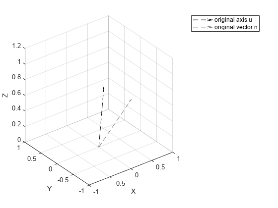
0. Initialization

Initialize the input vector and angle. u0 and n0 are the stored initial values of the axis $\overrightarrow{\underset{}{u}}$ and vector $$\overrightarrow{\underset{}{n}}$$.

clearvars
T = numerictype(1,16,13);
n0 = fi([sqrt(3)/2;0;1/2],T);
n = n0;
u0 = fi([sqrt(3)/3;sqrt(3)/3;sqrt(3)/3],T);
u = u0;
theta = fi(pi,T,'RoundingMethod','floor');

Configure the CORDIC rotation. Compute the maximum CORDIC shift value and inverse scale factor.

CORDICMaximumShiftValue = fixed.cordic.maximumShiftValue(u0);
Kn = fixed.cordic.circular.inverseScaleFactor(CORDICMaximumShiftValue);

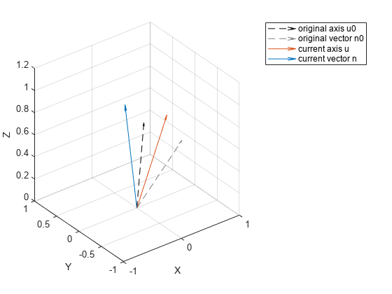
Plot the initial positions of vector $$\overrightarrow{\underset{}{n}}$$ and axis $\overrightarrow{\underset{}{u}}$ in three dimensions.

plotRot(u0,n0);

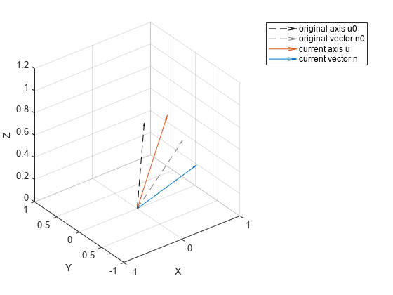
1. Rotate about X-axis to get $\overrightarrow{\underset{}{u}}$ into X-Z plane

Rotate $\overrightarrow{\underset{}{u}}$ and $$\overrightarrow{\underset{}{n}}$$ together about the X-axis to get $\overrightarrow{\underset{}{u}}$ into X-Z plane. V is $$\sqrt{u_z^2+u_y^2}$$.

[u(3),u(2),n(3),n(2)] = fixed.qr.cordicgivens(u0(3),u0(2),n(3),n(2),1,CORDICMaximumShiftValue,Kn);
V = u(3);

Plot the original and current positions.

plotRot(u0,n0,u,n,u0,n0)

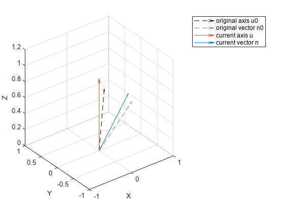
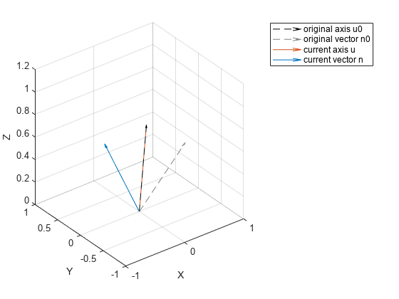
2. Rotate about Y-axis to get $\overrightarrow{\underset{}{u}}$ into Z direction

Rotate $\overrightarrow{\underset{}{u}}$ and $$\overrightarrow{\underset{}{n}}$$ together about the Y-axis to get $\overrightarrow{\underset{}{u}}$ into Z direction.

uprev = u;
nprev = n;
[u(3),u(1),n(1),n(3)] = fixed.qr.cordicgivens(u(3),-u(1),n(1),n(3),1,CORDICMaximumShiftValue,Kn);

Plot the original and current positions.

plotRot(u0,n0,u,n,uprev,nprev)

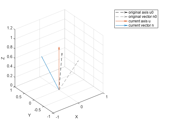
3. Rotate $$\overrightarrow{\underset{}{n}}$$ about Z-axis by $\theta$

Rotate the vector $$\overrightarrow{\underset{}{n}}$$ about the Z-axis by the angle $\theta$.

uprev = u;
nprev = n;
v = cordicRotateAngle([nprev(1),nprev(2)],theta,CORDICMaximumShiftValue,Kn);
n(1) = v(1);
n(2) = v(2);

Plot the original and current positions.

plotRot(u0,n0,u,n,uprev,nprev)

4. Reverse step 2

uprev = u;
nprev = n;
[~,~,n(1),n(3)] = fixed.qr.cordicgivens(V,u0(1),n(1),n(3),1,CORDICMaximumShiftValue,Kn);

Rotate $\overrightarrow{\underset{}{u}}$ for demonstration purposes.

[~,~,u(1),u(3)] = fixed.qr.cordicgivens(V,u0(1),u(1),u(3),1,CORDICMaximumShiftValue,Kn);

Plot the original and current positions.

plotRot(u0,n0,u,n,uprev,nprev)

5. Reverse step 1

uprev = u;
nprev = n;
[~,~,n(3),n(2)] = fixed.qr.cordicgivens(u0(3),-u0(2),n(3),n(2),1,CORDICMaximumShiftValue,Kn);
[~,~,u(3),u(2)] = fixed.qr.cordicgivens(u0(3),-u0(2),u(3),u(2),1,CORDICMaximumShiftValue,Kn);

Plot the original and current positions.

plotRot(u0,n0,u,n,uprev,nprev)

After 5 CORDIC rotations, the vector $$\overrightarrow{\underset{}{n}}$$ is rotated to the target direction and the rotation axis $\overrightarrow{\underset{}{u}}$ has returned to its original position.

u

u = 
    0.5775
    0.5776
    0.5774

          DataTypeMode: Fixed-point: binary point scaling
            Signedness: Signed
            WordLength: 16
        FractionLength: 13

u0

u0 = 
    0.5774
    0.5774
    0.5774

          DataTypeMode: Fixed-point: binary point scaling
            Signedness: Signed
            WordLength: 16
        FractionLength: 13

n

n = 
    0.0439
    0.9106
    0.4110

          DataTypeMode: Fixed-point: binary point scaling
            Signedness: Signed
            WordLength: 16
        FractionLength: 13

n0

n0 = 
    0.8660
         0
    0.5000

          DataTypeMode: Fixed-point: binary point scaling
            Signedness: Signed
            WordLength: 16
        FractionLength: 13

Implement CORDIC Rotation in Simulink for HDL Code Generation

The rotationAboutAxisModel Simulink® model contains a subsystem that shows how to implement this transformation. Additionally, this model is designed for HDL code generation.

model = 'rotationAboutAxisModel';
load_system(model);
open_system([model '/R']);

This model contains five CORDIC kernels corresponding to the five rotation steps described above. The CORDIC Rotate to Zero blocks use a circular vectoring mode to perform the rotations 1, 2, 4, and 5. The CORDIC Rotate by Angle block performs rotation step 3 using a circular rotation mode. The Unit Delay Enabled Synchronous blocks are used to model an internal buffer.

Simulate the Model

Configure the model workspace and simulate the model.

fixed.example.setModelWorkspace(model,'u',u0,'n',n0,'angle',theta,'numSamples',1);
out = sim(model);
nSim = out.nSim

nSim = 
    0.0437
    0.9106
    0.4111

          DataTypeMode: Fixed-point: binary point scaling
            Signedness: Signed
            WordLength: 16
        FractionLength: 13

Verify Result with Floating-Point Closed-Form Solution

As a reference for verification of the fixed-point model, compute the closed-form solution in floating point.

uf = double(u0);
c = cos(double(theta));  s = sin(double(theta));
c1 = 1 - c;
R = [c+uf(1)*uf(1)*c1, uf(1)*uf(2)*c1-uf(3)*s, uf(1)*uf(3)*c1+uf(2)*s; ...
     uf(1)*uf(2)*c1+uf(3)*s, c+uf(2)*uf(2)*c1, uf(2)*uf(3)*c1-uf(1)*s; ...
     uf(1)*uf(3)*c1-uf(2)*s, uf(2)*uf(3)*c1+uf(1)*s, c+uf(3)*uf(3)*c1];
nf = R*double(n0);
error = double(n)-nf;

Latency

This block is pipelined at the CORDIC rotation level. The expected throughput is wordlength+3 clock cycles.

expectedThroughput = u.WordLength+3

expectedThroughput = 19

The expected latency is (wordlength+2)*5 clock cycles.

expectedLatency = (u.WordLength+2)*5

expectedLatency = 90

Benchmark the throughput and latency from the simulation. The CORDIC rotation blocks in this model use the AMBA AXI handshaking process at both the input and output interfaces.

validInHistory = out.logsout.get('validIn').Values.Data;
validOutHistory = out.logsout.get('validOut').Values.Data;
readyHistory = out.logsout.get('ready').Values.Data;
readyInHistory = out.logsout.get('readyIn').Values.Data;

Block latency is defined as the number of clock cycles between an input and the corresponding output. Data input happens with both validIn and ready signals are asserted. Data output happens when both validOut and readyIn signals are asserted.

tDataIn = find(validInHistory & readyHistory == 1);
tDataOut = find(validOutHistory & readyInHistory == 1);
blockLatency = tDataOut - tDataIn(1:size(u,3))

blockLatency = 90

Throughput is defined as the data input and output rate.

blockThrougput = diff(tDataIn)

blockThrougput = 4×1

    19
    19
    19
    19

HDL Statistics

Both CORDIC rotation blocks in this example support HDL code generation using the Simulink® HDL Workflow Advisor. For an example, see HDL Code Generation and FPGA Synthesis from Simulink Model (HDL Coder)(HDL Coder) and Implement Digital Downconverter for FPGA (HDL Coder) (DSP HDL Toolbox).

This example data was generated by synthesizing the block on a Xilinx® Zynq®-7000 SoC ZC706 Evaluation Kit. The synthesis tool was Vivado® v2022.1 (win64).

These parameters were used for synthesis:

• Input data type: sfix16_En13

• maximumShiftValue: 15 (WordLength - 1)

• Target frequency: 200 MHz

This table shows the synthesis resource utilization results.

Resource	Usage	Available	Utilization (%)
Slice LUTs	2599	218600	1.19
Slice Registers	837	437200	0.19
DSPs	0	900	0.00
Block RAM Tile	0	545	0.00

This table shows the timing summary.

	Value
Requirement	5 ns (200 MHz)
Data Path Delay	4.463 ns
Slack	0.53 ns
Clock Frequency	223.71 MHz