Cast from Doubles to Fixed Point
This example shows you how to simulate a continuous real-world doubles signal using a
generalized fixed-point data type. Using the fxpdemo_dbl2fix model,
you can explore many of the important features of the Fixed-Point Designer™ software, including
Data types
Scaling
Rounding
Logging minimum and maximum simulation values to the workspace
Overflow handling
To open the model, at the MATLAB® command line, enter
openExample('fixedpoint/DoubleToFixedPointConversionExample')
In this example, you configure the Signal Generator block to output a sine wave signal with an amplitude
defined on the interval [-5 5]. The Signal Generator
block always outputs double-precision numbers.
The Dbl-to-FixPt
Data Type Conversion block converts the
double-precision numbers from the Signal Generator block into one of the
Fixed-Point Designer data types. For simplicity, the size of the output signal is 5 bits in
this example.
The FixPt-to-Dbl
Data Type Conversion block converts one of the Fixed-Point Designer data types into a Simulink® data type. In this example, it outputs double-precision numbers.
Simulate Using Binary-Point-Only Scaling
When using binary-point-only scaling, your goal is to find the fixed exponent, as defined in Binary-Point Scaling. For this scaling mode, the slope adjustment factor is 1 and there is no bias.
To set up the model to use binary-point-only scaling:
Configure the Signal Generator block to output a sine wave signal with an amplitude defined on the interval
[-5 5].Double-click the Signal Generator block to open the Block Parameters dialog box.
Set the Wave form parameter to
sine.Set the Amplitude parameter to
5.Click OK.
Configure the Data Type Conversion (Dbl-to-FixPt) block.
Double-click the Dbl-to-FixPt block to open the Block Parameters dialog box.
Verify that the Output data type parameter is
fixdt(1,5,2). This specifies a 5-bit, signed, fixed-point number with scaling2^-2, which puts the binary point two places to the left of the rightmost bit. Hence the maximum value is 011.11 = 3.75, the minimum value is 100.00 = -4.00, and the precision is (1/2)2 = 0.25.Verify that the Integer rounding mode parameter is set to
Floor. This rounds the fixed-point result toward negative infinity.Select the Saturate on integer overflow check box to prevent the block from wrapping on overflow.
Click OK.
To simulate the model, in the Simulation tab, click Run.
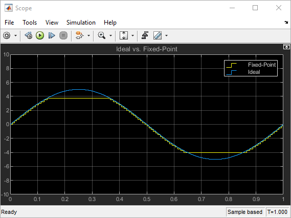
The Scope displays the ideal and the fixed-point simulation results.

The simulation shows the quantization effects of fixed-point arithmetic. Using a 5-bit word with a precision of (1/2)2 = 0.25 produces a discretized output that does not span the full range of the input signal.
To span the complete range of the input signal with 5 bits using binary-point-only
scaling, set the output scaling to 2^-1. This puts the binary
point one place to the left of the rightmost bit, giving a maximum value of 0111.1 =
7.5 and a minimum value of 1000.0 = -8.0. However, the precision is reduced to
(1/2)1 = 0.5. If you want to span the complete range
of the input signal with 5 bits using binary-point-only scaling, then your only
option is to sacrifice precision. Hence, the output scaling is
2^-1, which puts the binary point one place to the left of
the rightmost bit. This scaling gives a maximum value of 0111.1 = 7.5, a minimum
value of 1000.0 = -8.0, and a precision of (1/2)1 =
0.5.
To see the effect of reducing the precision to 0.5, set the Output data
type parameter of the Dbl-to-FixPt
Data Type Conversion block to fixdt(1,5,1) and
rerun the simulation.
Simulate Using Slope-Bias Scaling
When using slope-bias scaling, your goal is to find the optimal fractional slope
F and fixed power-of-two exponent E,
as defined in Slope-Bias Scaling. There is no bias for this example
because the sine wave is defined on the interval [-5 5].
To find the slope, you begin by assuming a fixed power-of-two exponent of -2. To
find the fractional slope, divide the maximum value of the sine wave by the maximum
value of the scaled 5-bit number. The result is 5.00/3.75 = 1.3333. The slope (and
precision) is 1.3333(0.25) = 0.3333. You specify the slope-bias scaling as [0.3333
0] by entering the expression fixdt(1,5,0.3333,0) as the value of
the Output data type parameter.
You could also specify a fixed power-of-two exponent of -1 and a corresponding fractional slope of 0.6667. The resulting slope is the same since the fixed exponent is reduced by 1 bit but the slope adjustment factor is increased by 1 bit. The Fixed-Point Designer software would automatically store the slope adjustment factor as 1.3332 and the fixed exponent as -2 because of the normalization condition of 1 ≤ F < 2.
To set up the model to use slope-bias scaling:
Configure the Signal Generator block to output a sine wave signal with an amplitude defined on the interval
[-5 5].Double-click the Signal Generator block to open the Block Parameters dialog box.
Set the Wave form parameter to
sine.Set the Amplitude parameter to
5.Click OK.
Configure the
Dbl-to-FixPtData Type Conversion block.Double-click the Dbl-to-FixPt block to open the Block Parameters dialog box.
To specify a slope-bias scaling of [0.3333 0], set the Output data type parameter to
fixdt(1,5,0.3333,0).Verify that the Integer rounding mode parameter is
Floor. This rounds the fixed-point result toward negative infinity.Select the Saturate on integer overflow check box to prevent the block from wrapping on overflow.
Click OK.
To simulate the model, in the Simulation tab, click Run.
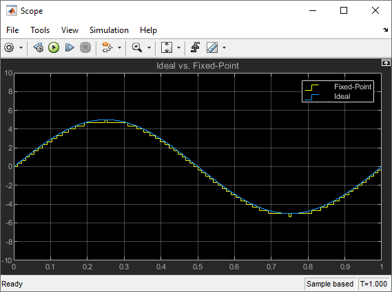
The Scope displays the ideal and the fixed-point simulation results.

If you do not know the slope, you can achieve reasonable simulation results by selecting your scaling based on the formula
where
max_value is the maximum value to be simulated
min_value is the minimum value to be simulated
ws is the word size in bits
2ws - 1 is the largest value of a word with size ws
For this example, the formula produces a slope of 0.32258.