Creating an IRFunctionCurve Object

To create an IRFunctionCurve object, see the following options:

• Fitting IRFunctionCurve Object Using a Function Handle

• Fitting IRFunctionCurve Object Using Nelson-Siegel Method

• Fitting IRFunctionCurve Object Using Svensson Method

• Fitting IRFunctionCurve Object Using Smoothing Spline Method

• Using fitFunction to Create Custom Fitting Function

Fitting IRFunctionCurve Object Using a Function Handle

You can use IRFunctionCurve with a MATLAB^® function handle to define an interest-rate curve. For more information on defining a function handle, see the MATLAB Programming Fundamentals documentation.

Example

This example uses a FunctionHandle argument with a value @(t) t.^2 to create an interest-rate curve.

rr = IRFunctionCurve('Zero',today,@(t) t.^2)

rr = 

  Properties:
    FunctionHandle: @(t)t.^2
              Type: 'Zero'
            Settle: 733600
       Compounding: 2
             Basis: 0

Fitting IRFunctionCurve Object Using Nelson-Siegel Method

This example shows how to use the function, fitNelsonSiegel, for the Nelson-Siegel model that fits the empirical form of the yield curve with a prespecified functional form of the spot rates which is a function of the time to maturity of the bonds.

The Nelson-Siegel model represents a dynamic three-factor model: level, slope, and curvature. However, the Nelson-Siegel factors are unobserved, or latent, which allows for measurement error, and the associated loadings have economic restrictions (forward rates are always positive, and the discount factor approaches zero as maturity increases). For more information, see "Zero-Coupon Yield Curves: Technical Documentation," BIS Papers, Bank for International Settlements, Number 25, October 2005.

This example uses IRFunctionCurve to model the default-free term structure of interest rates in the United Kingdom.

Load the data.

load ukdata20080430

Convert repo rates to be equivalent zero-coupon bonds.

RepoCouponRate = repmat(0,size(RepoRates));
RepoPrice = bndprice(RepoRates, RepoCouponRate, RepoSettle, RepoMaturity);

Aggregate the data.

Settle = [RepoSettle;BondSettle];
Maturity = [RepoMaturity;BondMaturity];
CleanPrice = [RepoPrice;BondCleanPrice];
CouponRate = [RepoCouponRate;BondCouponRate];
Instruments = [Settle Maturity CleanPrice CouponRate];
InstrumentPeriod = [repmat(0,6,1);repmat(2,31,1)];
CurveSettle = datetime(2008,4,30);

The IRFunctionCurve object provides the capability to fit a Nelson-Siegel curve to observed market data with the fitNelsonSiegel function. The fitting is done by calling the function lsqnonlin. The fitNelsonSiegel function has required inputs of Type, Settle, and a matrix of instrument data.

NSModel = IRFunctionCurve.fitNelsonSiegel('Zero',CurveSettle,...
Instruments,'Compounding',-1,'InstrumentPeriod',InstrumentPeriod);

Plot the Nelson-Siegel interest-rate curve for forward rates.

PlottingDates = CurveSettle+20:30:CurveSettle+365*25;
TimeToMaturity = yearfrac(CurveSettle,PlottingDates);
NSForwardRates = getForwardRates(NSModel, PlottingDates);
plot(TimeToMaturity,NSForwardRates)
title('Nelson Siegel Model of UK Instantaneous Nominal Forward Curve')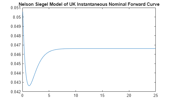

Fitting IRFunctionCurve Object Using Svensson Method

This example shows how to use the function, fitSvensson, for the Svensson model to improve the flexibility of the curves and the fit for a Nelson-Siegel model. In 1994, Svensson extended Nelson and Siegel's function by adding a further term that allows for a second "hump." The extra precision is achieved at the cost of adding two more parameters, ${\beta }_3^{}$amd ${\tau }_2^{}$, which have to be estimated.

This example of uses the fitSvensson function and an IRFitOptions structure, defined using IRFitOptions. Thus, you must specify FitType, InitialGuess, UpperBound, LowerBound, and the OptOptions optimization parameters for lsqnonlin.

Load the data.

load ukdata20080430

Convert repo rates to be equivalent zero coupon bonds.

RepoCouponRate = repmat(0,size(RepoRates));
RepoPrice = bndprice(RepoRates, RepoCouponRate, RepoSettle, RepoMaturity);

Aggregate the data.

Settle = [RepoSettle;BondSettle];
Maturity = [RepoMaturity;BondMaturity];
CleanPrice = [RepoPrice;BondCleanPrice];
CouponRate = [RepoCouponRate;BondCouponRate];
Instruments = [Settle Maturity CleanPrice CouponRate];
InstrumentPeriod = [repmat(0,6,1);repmat(2,31,1)];
CurveSettle = datetime(2008,4,30);

Define OptOptions for IRFitOptions.

OptOptions = optimoptions('lsqnonlin','MaxFunEvals',1000);
fIRFitOptions = IRFitOptions([5.82 -2.55 -.87 0.45 3.9 0.44],...
'FitType','durationweightedprice','OptOptions',OptOptions,...
'LowerBound',[0 -Inf -Inf -Inf 0 0],'UpperBound',[Inf Inf Inf Inf Inf Inf]);

Fit the interest-rate curve using a Svensson model.

SvenssonModel = IRFunctionCurve.fitSvensson('Zero',CurveSettle,...
Instruments,'IRFitOptions', fIRFitOptions, 'Compounding',-1,...
'InstrumentPeriod',InstrumentPeriod)

Local minimum possible.

lsqnonlin stopped because the final change in the sum of squares relative to 
its initial value is less than the value of the function tolerance.

<stopping criteria details>

SvenssonModel = 
			 Type: Zero
		   Settle: 733528 (30-Apr-2008)
	  Compounding: -1
			Basis: 0 (actual/actual)

The status message, output from lsqnonlin, indicates that the optimization to find parameters for the Svensson equation terminated successfully.

Plot the Svensson interest-rate curve for forward rates.

PlottingDates = CurveSettle+20:30:CurveSettle+365*25;
TimeToMaturity = yearfrac(CurveSettle,PlottingDates);
SvenssonForwardRates = getForwardRates(SvenssonModel, PlottingDates);
plot(TimeToMaturity,SvenssonForwardRates)
title('Svensson Model of UK Instantaneous Nominal Forward Curve')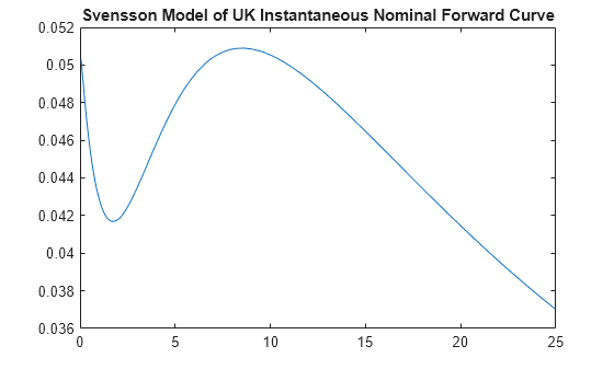

Fitting IRFunctionCurve Object Using Smoothing Spline Method

This example shows how to use fitSmoothingSpline to model the term structure with a spline, where the term structure represents the forward curve with a cubic spline.

Note: You must have a license for Curve Fitting Toolbox™ software to use the fitSmoothingSpline function.

The IRFunctionCurve object is used to fit a smoothing spline representation of the forward curve with a penalty function. Required inputs for fitSmoothingSpline are Type, Settle, the matrix of Instruments, and Lambdafun, a function handle containing the penalty function.

Load the data.

load ukdata20080430

Convert repo rates to be equivalent zero coupon bonds.

RepoCouponRate = repmat(0,size(RepoRates));
RepoPrice = bndprice(RepoRates, RepoCouponRate, RepoSettle, RepoMaturity);

Aggregate the data.

Settle = [RepoSettle;BondSettle];
Maturity = [RepoMaturity;BondMaturity];
CleanPrice = [RepoPrice;BondCleanPrice];
CouponRate = [RepoCouponRate;BondCouponRate];
Instruments = [Settle Maturity CleanPrice CouponRate];
InstrumentPeriod = [repmat(0,6,1);repmat(2,31,1)];
CurveSettle = datenum('30-Apr-2008');

Choose parameters for Lambdafun.

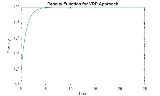
L = 9.2;
S = -1;
mu = 1;

Define the Lambdafun penalty function.

lambdafun = @(t) exp(L - (L-S)*exp(-t/mu));
t = 0:.1:25;
y = lambdafun(t);
figure
semilogy(t,y);
title('Penalty Function for VRP Approach')
ylabel('Penalty')
xlabel('Time')

Use the fitSmoothingSpline function to fit the interest-rate curve and model the Lambdafun penalty function.

VRPModel = IRFunctionCurve.fitSmoothingSpline('Forward',CurveSettle, ...
Instruments,lambdafun,'Compounding',-1, 'InstrumentPeriod',InstrumentPeriod);

Plot the smoothing spline interest-rate curve for forward rates.

PlottingDates = CurveSettle+20:30:CurveSettle+365*25;
TimeToMaturity = yearfrac(CurveSettle,PlottingDates);
VRPForwardRates = getForwardRates(VRPModel, PlottingDates);
plot(TimeToMaturity,VRPForwardRates)
title('Smoothing Spline Model of UK Instantaneous Nominal Forward Curve')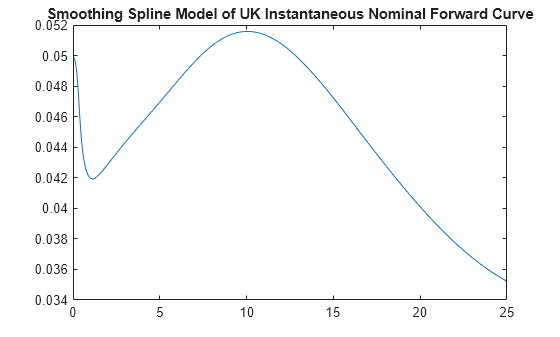

Using fitFunction to Create Custom Fitting Function

When using an IRFunctionCurve object, you can create a custom fitting function with the fitFunction function. To use fitFunction, you must define a FunctionHandle. In addition, you must also use IRFitOptions to define an IRFitOptions object to support an InitialGuess for the parameters of the curve function.

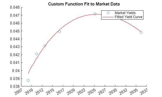
Create Custom Fitting Function

This example shows how to use fitFunction with a FunctionHandle and an IRFitOptions object.

Define the data.

Settle = repmat(datenum('30-Apr-2008'),[6 1]);
Maturity = [datenum('07-Mar-2009');datenum('07-Mar-2011'); ...
datenum('07-Mar-2013');datenum('07-Sep-2016'); ...
datenum('07-Mar-2025');datenum('07-Mar-2036')];

CleanPrice = [100.1;100.1;100.8;96.6;103.3;96.3];
CouponRate = [0.0400;0.0425;0.0450;0.0400;0.0500;0.0425];
Instruments = [Settle Maturity CleanPrice CouponRate];
CurveSettle = datenum('30-Apr-2008');

Define the FunctionHandle.

functionHandle = @(t,theta) polyval(theta,t);

Define the OptOptions for IRFitOptions.

OptOptions = optimoptions('lsqnonlin','display','iter');

Define fitFunction.

CustomModel = IRFunctionCurve.fitFunction('Zero', CurveSettle, ...
functionHandle,Instruments, IRFitOptions([.05 .05 .05],'FitType','price', ...
'OptOptions',OptOptions));

                                            Norm of      First-order 
 Iteration  Func-count      Resnorm            step       optimality
     0          4           38036.7                         4.92e+04
     1          8           38036.7              10         4.92e+04      
     2         12           38036.7             2.5         4.92e+04      
     3         16           38036.7           0.625         4.92e+04      
     4         20           38036.7         0.15625         4.92e+04      
     5         24           30741.5       0.0390625         1.72e+05      
     6         28           30741.5        0.078125         1.72e+05      
     7         32           30741.5       0.0195312         1.72e+05      
     8         36           28713.6      0.00488281         2.33e+05      
     9         40           20323.3      0.00976562         9.47e+05      
    10         44           20323.3       0.0195312         9.47e+05      
    11         48           20323.3      0.00488281         9.47e+05      
    12         52           20323.3       0.0012207         9.47e+05      
    13         56           19698.8     0.000305176         1.08e+06      
    14         60             17493     0.000610352            7e+06      
    15         64             17493       0.0012207            7e+06      
    16         68             17493     0.000305176            7e+06      
    17         72           15455.1     7.62939e-05         2.25e+07      
    18         76           15455.1     0.000177499         2.25e+07      
    19         80           13317.1      3.8147e-05         3.18e+07      
    20         84           12865.3     7.62939e-05         7.83e+07      
    21         88           11779.8     7.62939e-05         7.58e+06      
    22         92           11747.6     0.000152588         1.45e+05      
    23         96           11720.9     0.000305176         2.33e+05      
    24        100           11667.2     0.000610352         1.48e+05      
    25        104           11558.6       0.0012207         3.55e+05      
    26        108           11335.5      0.00244141         1.57e+05      
    27        112           10863.8      0.00488281         6.36e+05      
    28        116           9797.14      0.00976562         2.53e+05      
    29        120           6882.83       0.0195312         9.18e+05      
    30        124           6882.83       0.0373993         9.18e+05      
    31        128           3218.45      0.00934981         1.96e+06      
    32        132           612.703       0.0186996         3.01e+06      
    33        136           13.0998       0.0253882         3.05e+06      
    34        140         0.0762922      0.00154002         5.05e+04      
    35        144         0.0731652     3.61103e-06             29.9      
    36        148         0.0731652     6.32308e-08            0.063      

Local minimum possible.

lsqnonlin stopped because the final change in the sum of squares relative to 
its initial value is less than the value of the function tolerance.

<stopping criteria details>

Plot the custom function that is defined using fitFunction.

Yields = bndyield(CleanPrice,CouponRate,Settle(1),Maturity);
scatter(Maturity,Yields);
PlottingPoints = min(Maturity):30:max(Maturity);
hold on;
plot(PlottingPoints, getParYields(CustomModel, PlottingPoints),'r');
datetick
legend('Market Yields','Fitted Yield Curve')
title('Custom Function Fit to Market Data')