Plotting the Efficient Frontier for a Portfolio Object

This example shows how to use the plotFrontier function to create a plot of the efficient frontier for a given portfolio optimization problem. The plotFrontier function accepts several types of inputs and generates a plot with an optional possibility to output the estimates for portfolio risks and returns along the efficient frontier.

plotFrontier has four different ways that it can be used. In addition to a plot of the efficient frontier, if you have an initial portfolio in the InitPort property, plotFrontier also displays the return versus risk of the initial portfolio on the same plot. If you have a well-posed portfolio optimization problem set up in a Portfolio object and you use plotFrontier, you get a plot of the efficient frontier with the default number of portfolios on the frontier (the default number is 10 and is maintained in the hidden property defaultNumPorts). The following code illustrates a typical use of plotFrontier to create a new plot.

m = [ 0.05; 0.1; 0.12; 0.18 ];
C = [ 0.0064 0.00408 0.00192 0; 
      0.00408 0.0289 0.0204 0.0119;
      0.00192 0.0204 0.0576 0.0336;
      0 0.0119 0.0336 0.1225 ];
pwgt0 = [ 0.3; 0.3; 0.2; 0.1 ];
 
p = Portfolio('Name', 'Asset Allocation Portfolio', 'InitPort', pwgt0);
p = setAssetMoments(p, m, C);
p = setDefaultConstraints(p);
plotFrontier(p)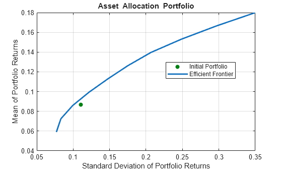

The Name property appears as the title of the efficient frontier plot if you set it in the Portfolio object. Without an explicit name, the title on the plot would be "Efficient Frontier." If you want to obtain a specific number of portfolios along the efficient frontier, use plotFrontier with the number of portfolios that you want. Suppose that you have the Portfolio object from the previous code and you want to plot 20 portfolios along the efficient frontier and to obtain 20 risk and return values for each portfolio.

[prsk, pret] = plotFrontier(p, 20);

display([pret, prsk])

    0.0590    0.0769
    0.0654    0.0784
    0.0718    0.0825
    0.0781    0.0890
    0.0845    0.0973
    0.0909    0.1071
    0.0972    0.1179
    0.1036    0.1296
    0.1100    0.1418
    0.1163    0.1545
    0.1227    0.1676
    0.1291    0.1810
    0.1354    0.1955
    0.1418    0.2128
    0.1482    0.2323
    0.1545    0.2535
    0.1609    0.2760
    0.1673    0.2995
    0.1736    0.3239
    0.1800    0.3500

Plotting Existing Efficient Portfolios

If you already have efficient portfolios from any of the "estimateFrontier" functions (see Estimate Efficient Portfolios for Entire Efficient Frontier for Portfolio Object), pass them into plotFrontier directly to plot the efficient frontier.

m = [ 0.05; 0.1; 0.12; 0.18 ];
C = [ 0.0064 0.00408 0.00192 0; 
      0.00408 0.0289 0.0204 0.0119;
      0.00192 0.0204 0.0576 0.0336;
      0 0.0119 0.0336 0.1225 ];
pwgt0 = [ 0.3; 0.3; 0.2; 0.1 ];
 
p = Portfolio('Name', 'Asset Allocation Portfolio', 'InitPort', pwgt0);
p = setAssetMoments(p, m, C);
p = setDefaultConstraints(p);
pwgt = estimateFrontier(p, 20);
plotFrontier(p, pwgt)

Plotting Existing Efficient Portfolio Risks and Returns

If you already have efficient portfolio risks and returns, you can use the interface to plotFrontier to pass them into plotFrontier to obtain a plot of the efficient frontier.

m = [ 0.05; 0.1; 0.12; 0.18 ];
C = [ 0.0064 0.00408 0.00192 0; 
      0.00408 0.0289 0.0204 0.0119;
      0.00192 0.0204 0.0576 0.0336;
      0 0.0119 0.0336 0.1225 ];
pwgt0 = [ 0.3; 0.3; 0.2; 0.1 ];
 
p = Portfolio('Name', 'Asset Allocation Portfolio', 'InitPort', pwgt0);
p = setAssetMoments(p, m, C);
p = setDefaultConstraints(p);
[prsk, pret] = estimatePortMoments(p, p.estimateFrontier(20));
plotFrontier(p, prsk, pret)