Plotting an Efficient Frontier Using portopt

This example shows how to use portopt to plot the efficient frontier of a hypothetical portfolio of three assets.

The following code plots the efficient frontier of a hypothetical portfolio of three assets. It illustrates how to specify the expected returns, standard deviations, and correlations of a portfolio of assets, how to convert standard deviations and correlations into a covariance matrix, and how to compute and plot the efficient frontier from the returns and covariance matrix. The example also illustrates how to randomly generate a set of portfolio weights, and how to add the random portfolios to an existing plot for comparison with the efficient frontier.

Specify the expected returns, standard deviations, and correlation matrix for a hypothetical portfolio of three assets.

Returns      = [0.1 0.15 0.12];
STDs         = [0.2 0.25 0.18];

Correlations = [ 1  0.3  0.4
                0.3  1   0.3
                0.4 0.3   1 ];

Convert the standard deviations and correlation matrix into a variance-covariance matrix with the function corr2cov.

Covariances = corr2cov(STDs, Correlations)

Covariances = 3×3

    0.0400    0.0150    0.0144
    0.0150    0.0625    0.0135
    0.0144    0.0135    0.0324

Evaluate and plot the efficient frontier at 20 points along the frontier, using the function portopt and the expected returns and corresponding covariance matrix. Although rather elaborate constraints can be placed on the assets in a portfolio, for simplicity accept the default constraints and scale the total value of the portfolio to 1 and constrain the weights to be positive (no short-selling).

Note: portopt has been partially removed and will no longer accept ConSet or varargin arguments. Use Portfolio object instead to solve portfolio problems that are more than a long-only fully-invested portfolio. For information on the workflow when using Portfolio objects, see Portfolio Object Workflow. For more information on migrating portopt code to Portfolio, see portopt Migration to Portfolio Object.

portopt(Returns, Covariances, 20)

Now that the efficient frontier is computed, randomly generate the asset weights for 1000 portfolios starting from the MATLAB® initial state.

rng('default')
Weights = rand(1000, 3);

The previous line of code generates three columns of uniformly distributed random weights, but does not guarantee they sum to 1. The following code segment normalizes the weights of each portfolio so that the total of the three weights represent a valid portfolio.

Total = sum(Weights, 2);     % Add the weights
Total = Total(:,ones(3,1));  % Make size-compatible matrix
Weights = Weights./Total;    % Normalize so sum = 1

Given the 1000 random portfolios created, compute the expected return and risk of each portfolio associated with the weights.

[PortRisk, PortReturn] = portstats(Returns, Covariances, Weights);

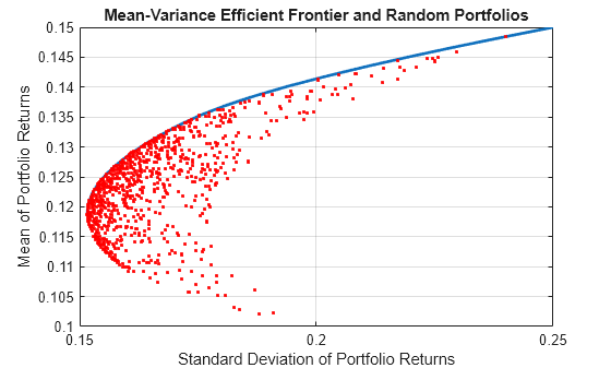
Plot the returns and risks of each portfolio on top of the existing efficient frontier for comparison. After plotting, annotate the graph with a title and return the graph to default holding status (any subsequent plots will erase the existing data). The efficient frontier appears in blue, while the 1000 random portfolios appear as a set of red dots on or below the frontier.

hold on
plot (PortRisk, PortReturn, '.r')
title('Mean-Variance Efficient Frontier and Random Portfolios')
hold off