Simulating Interest Rates

Simulate Interest Rates Through Interpolation

All simulation methods require that you specify a time grid by specifying the number of periods (NPeriods). You can also optionally specify a scalar or vector of strictly positive time increments (DeltaTime) and intermediate time steps (NSteps). These parameters, along with an initial sample time associated with the object (StartTime), uniquely determine the sequence of times at which the state vector is sampled. Thus, simulation methods allow you to traverse the time grid from beginning to end (that is, from left to right).

In contrast, interpolation methods allow you to traverse the time grid in any order, allowing both forward and backward movements in time. They allow you to specify a vector of interpolation times whose elements do not have to be unique.

Many references define the Brownian Bridge as a conditional simulation combined with a scheme for traversing the time grid, effectively merging two distinct algorithms. In contrast, the interpolation method offered here provides additional flexibility by intentionally separating the algorithms. In this method for moving about a time grid, you perform an initial Monte Carlo simulation to sample the state at the terminal time, and then successively sample intermediate states by stochastic interpolation. The first few samples determine the overall behavior of the paths, while later samples progressively refine the structure. Such algorithms are often called variance reduction techniques. This algorithm is simple when the number of interpolation times is a power of 2. In this case, each interpolation falls midway between two known states, refining the interpolation using a method like bisection. This example highlights the flexibility of refined interpolation by implementing this power-of-two algorithm.

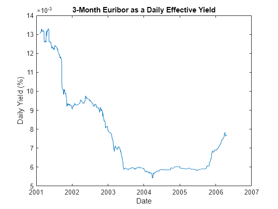
Load a historical data set of three-month Euribor rates, observed daily, and corresponding trading dates spanning the time interval from February 7, 2001 through April 24, 2006.

load Data_GlobalIdx2
plot(dates, 100 * Dataset.EB3M)
datetick('x'), xlabel('Date'), ylabel('Daily Yield (%)')
title('3-Month Euribor as a Daily Effective Yield')

Fit a simple univariate Vasicek model to the daily equivalent yields of the three-month Euribor data:

Given initial conditions, the distribution of the short rate at some time T in the future is Gaussian with mean:

and variance:

To calibrate this simple short-rate model, rewrite it in more familiar regression format:

where:

perform an ordinary linear regression where the model volatility is proportional to the standard error of the residuals:

yields     = Dataset.EB3M;
regressors = [ones(length(yields) - 1, 1) yields(1:end-1)];
[coefficients, intervals, residuals] = ...
   regress(diff(yields), regressors);
dt    = 1;  % time increment = 1 day
speed = -coefficients(2)/dt;
level = -coefficients(1)/coefficients(2);
sigma =  std(residuals)/sqrt(dt);

Create an hwv object with StartState set to the most recently observed short rate.

obj = hwv(speed, level, sigma, 'StartState', yields(end))

obj = 
   Class HWV: Hull-White/Vasicek
   ----------------------------------------
     Dimensions: State = 1, Brownian = 1
   ----------------------------------------
      StartTime: 0
     StartState: 7.70408e-05
    Correlation: 1
          Drift: drift rate function F(t,X(t)) 
      Diffusion: diffusion rate function G(t,X(t)) 
     Simulation: simulation method/function simByEuler
          Sigma: 4.77637e-07
          Level: 6.00424e-05
          Speed: 0.00228854

Assume, for example, that you simulate the fitted model over 64 ($2_{}^6$) trading days, using a refined Brownian bridge with the power-of-two algorithm instead of the usual beginning-to-end Monte Carlo simulation approach. Furthermore, assume that the initial time and state coincide with those of the last available observation of the historical data, and that the terminal state is the expected value of the Vasicek model 64 days into the future. In this case, you can assess the behavior of various paths that all share the same initial and terminal states, perhaps to support pricing path-dependent interest rate options over a three-month interval.

Create a vector of interpolation times to traverse the time grid by moving both forward and backward in time. Specifically, the first interpolation time is set to the most recent short-rate observation time, the second interpolation time is set to the terminal time, and subsequent interpolation times successively sample intermediate states.

T      = 64;
times  = (1:T)';
t      = NaN(length(times) + 1, 1);
t(1)   = obj.StartTime;
t(2)   = T;
delta  = T;
jMax   = 1;
iCount = 3;

for k = 1:log2(T)
    i = delta / 2;
    for j = 1:jMax
        t(iCount) = times(i);
        i         = i + delta;
        iCount    = iCount + 1;
    end
    jMax  = 2 * jMax;
    delta = delta / 2;
end

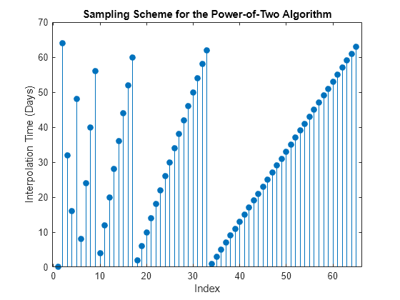
Plot the interpolation times to examine the sequence of interpolation times generated by this algorithm.

stem(1:length(t), t, 'filled')
xlabel('Index'), ylabel('Interpolation Time (Days)')
title ('Sampling Scheme for the Power-of-Two Algorithm')

The first few samples are widely separated in time and determine the course structure of the paths. Later samples are closely spaced and progressively refine the detailed structure.

Now that you have generated the sequence of interpolation times, initialize a course time series grid to begin the interpolation. The sampling process begins at the last observed time and state taken from the historical short-rate series, and ends 64 days into the future at the expected value of the Vasicek model derived from the calibrated parameters.

average = obj.StartState * exp(-speed * T) + level * ...
(1 - exp(-speed * T));
X       = [obj.StartState ; average];

Generate five sample paths, setting the Refine input flag to TRUE to insert each new interpolated state into the time series grid as it becomes available. Perform interpolation on a trial-by-trial basis. Because the input time series X has five trials (where each page of the three-dimensional time series represents an independent trial), the interpolated output series Y also has five pages.

nTrials = 5;
rng(63349,'twister')
Y = obj.interpolate(t, X(:,:,ones(nTrials,1)), ...
'Times',[obj.StartTime  T], 'Refine', true);

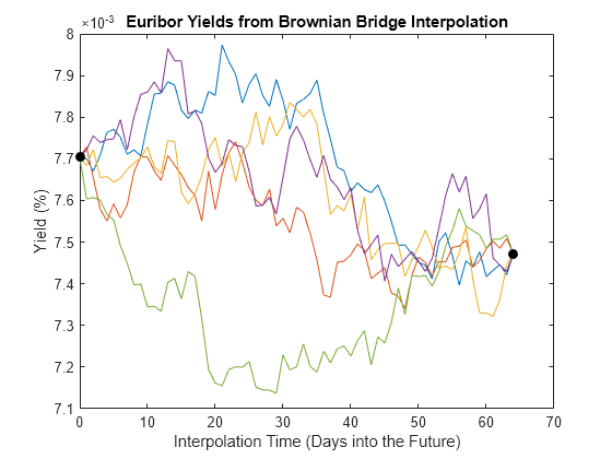
Plot the resulting sample paths. Because the interpolation times do not monotonically increase, sort the times and reorder the corresponding short rates.

[t,i] = sort(t);
Y     = squeeze(Y);
Y     = Y(i,:);
plot(t, 100 * Y), hold('on')
plot(t([1 end]), 100 * Y([1 end],1),'. black','MarkerSize',20)
xlabel('Interpolation Time (Days into the Future)')
ylabel('Yield (%)'), hold('off')
title ('Euribor Yields from Brownian Bridge Interpolation')

The short rates in this plot represent alternative sample paths that share the same initial and terminal values. They illustrate a special, though simplistic, case of a broader sampling technique known as stratified sampling. For a more sophisticated example of stratified sampling, see Stratified Sampling.

Although this simple example simulated a univariate Vasicek interest rate model, it applies to problems of any dimensionality. Brownian-bridge methods also apply more general variance-reduction techniques. For more information, see Stratified Sampling.

Simulate Positive Interest Rates

All simulation and interpolation methods allow you to specify a sequence of functions, or background processes, to evaluate at the end of every sample time period. This period includes any intermediate time steps determined by the optional NSteps input, as discussed in Optimizing Accuracy: About Solution Precision and Error. These functions are specified as callable functions of time and state, and must return an updated state vector ${\mathit{X}}_{\mathit{t}}^{}$as follows:

You must specify multiple processing functions as a cell array of functions. These functions are invoked in the order in which they appear in the cell array.

Processing functions are not required to use time (t) or state (${\mathit{X}}_{\mathit{t}}^{}$). They are also not required to update or change the input state vector. In fact, simulation and interpolation methods have no knowledge of any implementation details, and in this respect, they only adhere to a published interface.

Such processing functions provide a powerful modeling tool that can solve various problems. Such functions allow you to, for example, specify boundary conditions, accumulate statistics, plot graphs, and price path-dependent options.

Except for Brownian motion (BM) models, the individual components of the simulated state vector typically represent variables whose real-world counterparts are inherently positive quantities, such as asset prices or interest rates. However, by default, most of the simulation and interpolation methods provided here model the transition between successive sample times as a scaled (possibly multivariate) Gaussian draw. So, when approximating a continuous-time process in discrete time, the state vector may not remain positive. The only exception is simBySolution for gbm objects and simBySolution for hwv objects, a logarithmic transform of separable geometric Brownian motion models. Moreover, by default, none of the simulation and interpolation methods make adjustments to the state vector. Therefore, you are responsible for ensuring that all components of the state vector remain positive as appropriate.

Fortunately, specifying nonnegative states ensures a simple end-of-period processing adjustment. Although this adjustment is widely applicable, it is revealing when applied to a univariate cir square-root diffusion model:

Perhaps the primary appeal of univariate cir models where:

is that the short rate remains positive. However, the positivity of short rates only holds for the underlying continuous-time model.

To illustrate the latter statement, simulate daily short rates of the cir model, using cir, over one calendar year (approximately 250 trading days).

rng(14151617,'twister')
obj   = cir(0.25,@(t,X)0.1,0.2,'StartState',0.02);
[X,T] = simByEuler(obj,250,'DeltaTime',1/250,'nTrials',5);
sprintf('%0.4f\t%0.4f+i%0.4f\n',[T(195:205)';...
    real(X(195:205,1,4))'; imag(X(195:205,1,4))'])

ans = 
    '0.7760	0.0003+i0.0000
     0.7800	0.0004+i0.0000
     0.7840	0.0002+i0.0000
     0.7880	-0.0000+i0.0000
     0.7920	0.0001+i0.0000
     0.7960	0.0002+i0.0000
     0.8000	0.0002+i0.0000
     0.8040	0.0008+i0.0001
     0.8080	0.0004+i0.0001
     0.8120	0.0008+i0.0001
     0.8160	0.0008+i0.0001
     '

Interest rates can become negative if the resulting paths are simulated in discrete time. Moreover, since cir models incorporate a square root diffusion term, the short rates might even become complex.

Repeat the simulation, this time specifying a processing function that takes the absolute magnitude of the short rate at the end of each period. You can access the processing function by time and state $\left(\mathit{t},{\mathit{X}}_{\mathit{t}}^{}\right)$, but it only uses the state vector of short rates ${\mathit{X}}_{\mathit{t}}^{}.$

rng(14151617,'twister')
[Y,T] = simByEuler(obj,250,'DeltaTime',1/250,... 
    'nTrials',5,'Processes',@(t,X)abs(X));

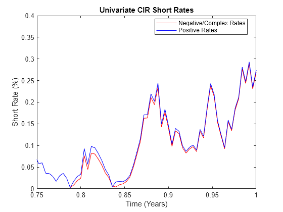
Graphically compare the magnitude of the unadjusted path (with negative and complex numbers) to the corresponding path kept positive by using an end-of-period processing function over the time span of interest.

clf
plot(T,100*abs(X(:,1,4)),'red',T,100*Y(:,1,4),'blue')
axis([0.75 1 0 0.4])
xlabel('Time (Years)'), ylabel('Short Rate (%)')
title('Univariate CIR Short Rates')
legend({'Negative/Complex Rates' 'Positive Rates'}, ... 
    'Location', 'Best')

You can use this method to obtain more accurate SDE solutions. For more information, see Performance Considerations.