Time Base Partitions for ARIMA Model Estimation
When you fit a time series model to data, lagged terms in the model require initialization, usually with observations at the beginning of the sample. Also, to measure the quality of forecasts from the model, you must hold out data at the end of your sample from estimation. Therefore, before analyzing the data, partition the time base into three consecutive, disjoint intervals:
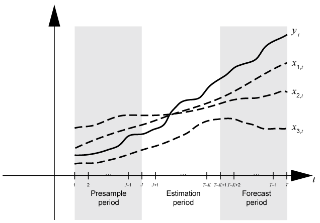
Three time base partitions for univariate autoregressive integrated moving average (ARIMA) models are the presample, estimation, and forecast periods.
Presample period — Contains data used to initialize lagged values in the model. An autoregressive integrated moving average model ARIMA(p,D,q)⨉(ps,Ds,qs)s model requires a presample period containing at least p + D + ps + s observations (see property P of the
arimamodel object). For example, if you plan to fit an ARIMA(4,1,1) model, the conditional expected value of Δyt, given its history, contains Δyt – 1 = yt – 1 – yt – 2 through Δyt – 4 = yt – 4 – yt – 5. The conditional expected value of Δy6 is a function of y5 through y1 and, therefore, the likelihood contribution of Δy6 requires those observations. Also, data does not exist for the likelihood contributions of Δy1 through Δy5. Therefore, model estimation requires a presample period of at least five time points.Estimation period — Contains the observations to which the model is explicitly fit. The number of observations in the estimation sample is the effective sample size. For parameter identifiability, the effective sample size should be at least the number of parameters being estimated.
Forecast period — Optional period during which forecasts are generated, known as the forecast horizon. This partition contains holdout data for model predictability validation.
Suppose yt is a response
series and Xt is a 3-D
exogenous series. Consider fitting a
SARIMAX(p,D,q)⨉(ps,Ds,qs)s
model of yt to the response
data in the T-by-1 vector y and the exogenous data
in the T-by-3 matrix X. Also, you want the
forecast horizon to have length K (that is, you want to hold out
K observations at the end of the sample to compare to the
forecasts from the fitted model).
This figure shows the time base partitions for model estimation. In the figure, J = p + D + ps + s.
This figure shows portions of the arrays that correspond to input arguments of the
estimate function of the
arima model.
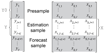
Yis the required input for specifying the response data to which the model is fit.'Y0'is an optional name-value pair argument for specifying the presample response data.Y0must have at least J rows. To initialize the model,estimateuses only the latest J observationsY0((end –.J+ 1):end)estimatealso accepts presample innovations and conditional variances when you specify the 'E0'and'V0'name-value pair arguments. These series are not included in the figures, but the same principles extend to them.'X'is an optional name-value pair argument for specifying exogenous data for the regression component. By default,estimateexcludes a regression component from the model, regardless of the value of the regression coefficientBetain thearimamodel template.
For a model without an exogenous regression component, if you do not specify
Y0, estimate backcasts the model for the
required presample observations. estimate subsequently fits the
model to the entire specified response data Y. Although
estimate backcasts for the presample by default, you can
extract the presample from the data and specify it using the 'Y0'
name-value pair argument to ensure that estimate initializes and
fits the model to your specifications.
If you specify 'X', the following conditions apply:
estimatesynchronizesXandywith respect to the last observation in the arrays (T – K in the previous figure), and applies only the required number of observations to the regression component. This action implies thatXcan have more rows thanY.If you do not specify
'Y0', you must supply at least J more exogenous observations than responses.estimateuses the extra presample exogenous data to backcast the model for presample responses.If you specify
'Y0',estimateuses only the latest exogenous observations required to fit the model (observations J + 1 through T – K in the previous figure).estimateignores presample exogenous data.
If you plan to validate the predictive power of the fitted model, you must extract the forecast sample from your data set before estimation.
Partition Time Series Data for Estimation
This example shows how to partition the time base of the monthly international airline passenger data set Data_Airline to initialize estimation and assess the predictive performance of the estimated model.
Load and Preprocess Data
Load the data.
load Data_AirlineThe variable DataTimeTable is a timetable containing the time series PSSG.
Plot the time series.
plot(DataTimeTable.Time,DataTable.PSSG)
xlabel('Time (months)')
ylabel('Passenger Counts')

The series exhibits seasonality and an exponential trend.
Determine whether the data has any missing values.
anymissing = sum(ismissing(DataTable))
anymissing = 1×2

     0     0
No missing observations are present.
Stabilize the series by applying the log transform.
StblTT = varfun(@log,DataTimeTable);
Partition Time Base
Consider a SARIMA model for the log of the monthly passenger counts from 1949 through 1960. The model requires presample responses. An arima model template for estimation stores the required number of presample responses in the property P.
Create a SARIMA model template for estimation. Specify that the model constant is 0. Verify the required number of presample observations by displaying the value of P using dot notation.
Mdl = arima('Constant',0,'D',1,'MALags',1,'SMALags',12,...
    'Seasonality',12);
Mdl.P
ans =
13
Consider a forecast horizon of two years (24 months). Partition the response data into presample, estimation, and forecast sample variables.
fh = 24;                % Forecast horizon
T = size(StblTT,1);     % Total sample size
eT = T - Mdl.P - fh;    % Effective sample size

idxpre = 1:Mdl.P;
idxest = (Mdl.P + 1):(T - fh);
idxfor = (T - fh + 1):T;

y0 = StblTT.log_PSSG(idxpre);  % Presample responses
y = StblTT.log_PSSG(idxest);   % Estimation sample responses
yf = StblTT.log_PSSG(idxfor);  % Forecast sample responses
Estimate Model
Fit the model to the estimation sample. Specify the presample by using the 'Y0' name-value pair argument.
EstMdl = estimate(Mdl,y,'Y0',y0);
    ARIMA(0,1,1) Model Seasonally Integrated with Seasonal MA(12) (Gaussian Distribution):

                  Value      StandardError    TStatistic      PValue
                _________    _____________    __________    __________

    Constant            0              0           NaN             NaN
    MA{1}        -0.31781       0.087289       -3.6408      0.00027175
    SMA{12}      -0.56707        0.10111       -5.6083      2.0434e-08
    Variance    0.0014446     0.00018295        7.8962      2.8763e-15
EstMdl is a fully specified arima model representing the estimated SARIMA model
where is Gaussian with a mean of 0 and a variance of 0.0019.
Because the constant is 0 in the model template, estimate treats it as an equality constraint during optimization. Therefore, inferences on the constant are irrelevant.
You can forecast the model using the forecast function of arima by specifying EstMdl and the forecast horizon fh. To initialize the model for forecasting, specify the estimation sample response data y by using the 'Y0' name-value pair argument.