Seasonal Adjustment Using a Stable Seasonal Filter

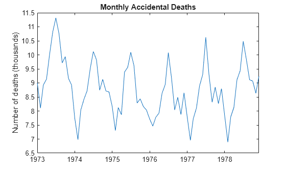
This example shows how to use a stable seasonal filter to deseasonalize a time series (using an additive decomposition). The time series is monthly accidental deaths in the U.S. from 1973 to 1978 (Brockwell and Davis, 2002).

Load Data

Load the accidental deaths data set.

load Data_Accidental
y = DataTimeTable.NUMD;
T = length(y);

figure
plot(DataTimeTable.Time,y/1000)
title('Monthly Accidental Deaths')
ylabel('Number of deaths (thousands)')
hold on

The data exhibits a strong seasonal component with periodicity 12.

Apply 13-term moving average

Smooth the data using a 13-term moving average. To prevent observation loss, repeat the first and last smoothed values six times. Subtract the smoothed series from the original series to detrend the data. Add the moving average trend estimate to the observed time series plot.

sW13 = [1/24; repmat(1/12,11,1); 1/24];
yS = conv(y,sW13,'same');
yS(1:6) = yS(7); yS(T-5:T) = yS(T-6);

xt = y-yS;

plot(DataTimeTable.Time,yS/1000,'r','LineWidth',2);
legend('13-Term Moving Average')
hold off

The detrended time series is xt.

Using the shape parameter 'same' when calling conv returns a smoothed series the same length as the original series.

Create Seasonal Indices

Create a cell array, sidx, to store the indices corresponding to each period. The data is monthly, with periodicity 12, so the first element of sidx is a vector with elements 1, 13, 25,...,61 (corresponding to January observations). The second element of sidx is a vector with elements 2, 14, 16,...,62 (corresponding to February observations). This is repeated for all 12 months.

s = 12;
sidx = cell(s,1);
for i = 1:s
 sidx{i,1} = i:s:T;
end

sidx{1:2}

ans = 1×6

     1    13    25    37    49    61

ans = 1×6

     2    14    26    38    50    62

Using a cell array to store the indices allows for the possibility that each period does not occur the same number of times within the span of the observed series.

Apply Stable Seasonal Filter

Apply a stable seasonal filter to the detrended series, xt. Using the indices constructed in Step 3, average the detrended data corresponding to each period. That is, average all of the January values (at indices 1, 13, 25,...,61), and then average all of the February values (at indices 2, 14, 26,...,62), and so on for the remaining months. Put the smoothed values back into a single vector.

Center the seasonal estimate to fluctuate around zero.

sst = cellfun(@(x) mean(xt(x)),sidx);

% Store smoothed values in a vector of length T
nc = floor(T/s);    % Num. complete years
rm = mod(T,s);      % Num. extra months
sst = [repmat(sst,nc,1);sst(1:rm)];

% Center the seasonal estimate (additive)
sBar = mean(sst); 
sst = sst-sBar;

figure
plot(DataTimeTable.Time,sst/1000)
title('Stable Seasonal Component')
ylabel('Number of deaths (thousands)')

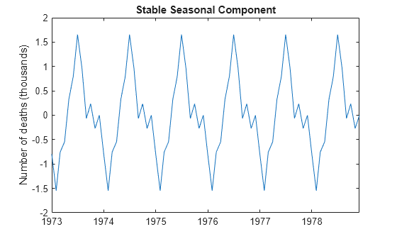
The stable seasonal component has constant amplitude across the series. The seasonal estimate is centered, and fluctuates around zero.

Deseasonalize Series

Subtract the estimated seasonal component from the original data.

dt = y - sst;

figure
plot(DataTimeTable.Time,dt/1000)
title('Deseasonalized Series')
ylabel('Number of deaths (thousands)')

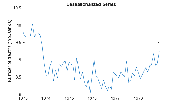
The deseasonalized series consists of the long-term trend and irregular components. A large-scale quadratic trend in the number of accidental deaths is clear with the seasonal component removed.

References:

Brockwell, P. J. and R. A. Davis. Introduction to Time Series and Forecasting. 2nd ed. New York, NY: Springer, 2002.