Plot Impulse Response of Regression Model with ARIMA Errors

Impulse response functions help examine the effects of a unit innovation shock to future values of the response of a time series model, without accounting for the effects of exogenous predictors. For example, if an innovation shock to an aggregate output series, e.g., GDP, is persistent, then GDP is sensitive to such shocks. The examples below show how to plot impulse response functions for regression models with various ARIMA error model structures using impulse.

Regression Model with AR Errors

This example shows how to plot the impulse response function for a regression model with AR errors.

Specify the regression model with AR(4) errors:

$$\begin{array}{l}{y}_t=2+X_t\left[\begin{array}{l}5\\ -1\end{array}\right]+u_t\\ u_t=0.9u_{t-1}-0.8u_{t-2}+0.75u_{t-3}-0.6u_{t-4}+{\epsilon }_t.\end{array}$$

Mdl = regARIMA('Intercept',2,'Beta',[5; -1],'AR',...
    {0.9, -0.8, 0.75, -0.6})

Mdl = 
  regARIMA with properties:

     Description: "Regression with ARMA(4,0) Error Model (Gaussian Distribution)"
      SeriesName: "Y"
    Distribution: Name = "Gaussian"
       Intercept: 2
            Beta: [5 -1]
               P: 4
               Q: 0
              AR: {0.9 -0.8 0.75 -0.6} at lags [1 2 3 4]
             SAR: {}
              MA: {}
             SMA: {}
        Variance: NaN

The dynamic multipliers are absolutely summable because the autoregressive component is stable. Therefore, Mdl is stationary.

You do not need to specify the innovation variance.

Plot the impulse response function.

impulse(Mdl)

The impulse response decays to 0 since Mdl defines a stationary error process. The regression component does not impact the impulse responses.

Regression Model with MA Errors

This example shows how to plot a regression model with MA errors.

Specify the regression model with MA(10) errors:

$$\begin{array}{l}{y}_t=2+X_t\left[\begin{array}{l}5\\ -1\end{array}\right]+u_t\\ u_t={\epsilon }_t+0.5{\epsilon }_{t-2}-0.4{\epsilon }_{t-4}-0.3{\epsilon }_{t-6}+0.2{\epsilon }_{t-8}-0.1{\epsilon }_{t-10}.\end{array}$$

Mdl = regARIMA('Intercept',2,'Beta',[5; -1],...
    'MA',{0.5,-0.4,-0.3,0.2,-0.1},'MALags',[2 4 6 8 10])

Mdl = 
  regARIMA with properties:

     Description: "Regression with ARMA(0,10) Error Model (Gaussian Distribution)"
      SeriesName: "Y"
    Distribution: Name = "Gaussian"
       Intercept: 2
            Beta: [5 -1]
               P: 0
               Q: 10
              AR: {}
             SAR: {}
              MA: {0.5 -0.4 -0.3 0.2 -0.1} at lags [2 4 6 8 10]
             SMA: {}
        Variance: NaN

The dynamic multipliers are absolutely summable because the moving average component is invertible. Therefore, Mdl is stationary.

You do not need to specify the innovation variance.

Plot the impulse response function for 10 responses.

impulse(Mdl,10)

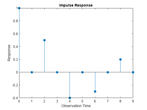
The impulse response of an MA error model is simply the MA coefficients at their corresponding lags.

Regression Model with ARMA Errors

This example shows how to plot the impulse response function of a regression model with ARMA errors.

Specify the regression model with ARMA(4,10) errors:

$$\begin{array}{c}{y}_t=2+X_t\left[\begin{array}{l}5\\ -1\end{array}\right]+u_t\\ \left(1-0.9L+0.8L^2-0.75L^3+0.6L^4\right)u_t=\left(1+0.5L^2-0.4L^4-0.3L^6+0.2L^8-0.1L^{10}\right)\end{array}$$

Mdl = regARIMA('Intercept',2,'Beta',[5; -1],...
    'AR',{0.9, -0.8, 0.75, -0.6},...
    'MA',{0.5, -0.4, -0.3, 0.2, -0.1},'MALags',[2 4 6 8 10])

Mdl = 
  regARIMA with properties:

     Description: "Regression with ARMA(4,10) Error Model (Gaussian Distribution)"
      SeriesName: "Y"
    Distribution: Name = "Gaussian"
       Intercept: 2
            Beta: [5 -1]
               P: 4
               Q: 10
              AR: {0.9 -0.8 0.75 -0.6} at lags [1 2 3 4]
             SAR: {}
              MA: {0.5 -0.4 -0.3 0.2 -0.1} at lags [2 4 6 8 10]
             SMA: {}
        Variance: NaN

The dynamic multipliers are absolutely summable because the autoregressive component is stable, and the moving average component is invertible. Therefore, Mdl defines a stationary error process.

You do not need to specify the innovation variance.

Plot the first 30 impulse responses.

impulse(Mdl,30)

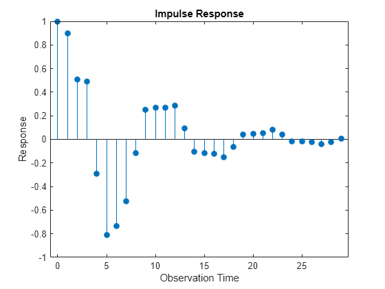
The impulse response decays to 0 since Mdl defines a stationary error process.

Regression Model with ARIMA Errors

This example shows how to plot the impulse response function of a regression model with ARIMA errors.

Specify the regression model with ARIMA(4,1,10) errors:

$$\begin{array}{c}{y}_t=2+X_t\left[\begin{array}{l}5\\ -1\end{array}\right]+u_t\\ \left(1-0.9L+0.8L^2-0.75L^3+0.6L^4\right)(1-L)u_t=\left(1+0.5L^2-0.4L^4-0.3L^6+0.2L^8-0.1L^{10}\right){\epsilon }_t.\end{array}$$

Mdl = regARIMA('Intercept',2,'Beta',[5; -1],...
    'AR',{0.9, -0.8, 0.75, -0.6},...
    'MA',{0.5, -0.4, -0.3, 0.2, -0.1},...
    'MALags',[2 4 6 8 10],'D',1)

Mdl = 
  regARIMA with properties:

     Description: "Regression with ARIMA(4,1,10) Error Model (Gaussian Distribution)"
      SeriesName: "Y"
    Distribution: Name = "Gaussian"
       Intercept: 2
            Beta: [5 -1]
               P: 5
               D: 1
               Q: 10
              AR: {0.9 -0.8 0.75 -0.6} at lags [1 2 3 4]
             SAR: {}
              MA: {0.5 -0.4 -0.3 0.2 -0.1} at lags [2 4 6 8 10]
             SMA: {}
        Variance: NaN

One of the roots of the compound autoregressive polynomial is 1, therefore Mdl defines a nonstationary error process.

You do not need to specify the innovation variance.

Plot the first impulse responses.

quot = sum([1,cell2mat(Mdl.MA)])/sum([1,-cell2mat(Mdl.AR)])

quot = 1.2000

impulse(Mdl,50)
hold on
plot([1 50],[quot quot],'r--','Linewidth',2.5)
hold off

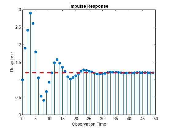
The impulse responses do not decay to 0. They settle at the quotient of the sums of the moving average and autoregressive polynomial coefficients (quot).

$$\text{quot}=\frac{1+0.5-0.4-0.3+0.2-0.1}{1-0.9+0.8-0.75+0.6}=1.2.$$