Forecast State-Space Model Observations
This example shows how to forecast observations of a known, time-invariant, state-space model.
Suppose that a latent process is an AR(1). The state equation is
where is Gaussian with mean 0 and standard deviation 1.
Generate a random series of 100 observations from , assuming that the series starts at 1.5.
T = 100;
ARMdl = arima('AR',0.5,'Constant',0,'Variance',1);
x0 = 1.5;
rng(1); % For reproducibility
x = simulate(ARMdl,T,'Y0',x0);
Suppose further that the latent process is subject to additive measurement error. The observation equation is
where is Gaussian with mean 0 and standard deviation 0.75. Together, the latent process and observation equations compose a state-space model.
Use the random latent state process (x) and the observation equation to generate observations.
y = x + 0.75*randn(T,1);
Specify the four coefficient matrices.
A = 0.5;
B = 1;
C = 1;
D = 0.75;
Specify the state-space model using the coefficient matrices.
Mdl = ssm(A,B,C,D)
Mdl =
State-space model type: ssm

State vector length: 1
Observation vector length: 1
State disturbance vector length: 1
Observation innovation vector length: 1
Sample size supported by model: Unlimited

State variables: x1, x2,...
State disturbances: u1, u2,...
Observation series: y1, y2,...
Observation innovations: e1, e2,...

State equation:
x1(t) = (0.50)x1(t-1) + u1(t)

Observation equation:
y1(t) = x1(t) + (0.75)e1(t)

Initial state distribution:

Initial state means
 x1
  0

Initial state covariance matrix
     x1
 x1  1.33

State types
     x1
 Stationary
Mdl is an ssm model. Verify that the model is correctly specified using the display in the Command Window. The software infers that the state process is stationary. Subsequently, the software sets the initial state mean and covariance to the mean and variance of the stationary distribution of an AR(1) model.
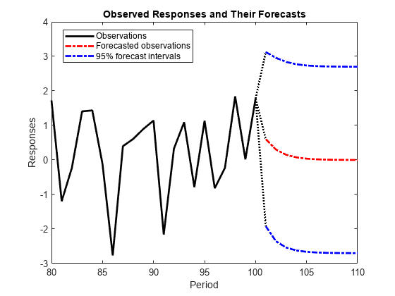
Forecast the observations 10 periods into the future, and estimate their variances.
numPeriods = 10;
[ForecastedY,YMSE] = forecast(Mdl,numPeriods,y);
Plot the forecasts with the in-sample responses, and 95% Wald-type forecast intervals.
ForecastIntervals(:,1) = ForecastedY - 1.96*sqrt(YMSE);
ForecastIntervals(:,2) = ForecastedY + 1.96*sqrt(YMSE);

figure
plot(T-20:T,y(T-20:T),'-k',T+1:T+numPeriods,ForecastedY,'-.r',...
    T+1:T+numPeriods,ForecastIntervals,'-.b',...
    T:T+1,[y(end)*ones(3,1),[ForecastedY(1);ForecastIntervals(1,:)']],':k',...
    'LineWidth',2)
hold on
title({'Observed Responses and Their Forecasts'})
xlabel('Period')
ylabel('Responses')
legend({'Observations','Forecasted observations','95% forecast intervals'},...
    'Location','Best')
hold off
See Also
Topics
- Create Continuous State-Space Models for Economic Data Analysis
- What Is the Kalman Filter?
- Model Local Trends in Global Carbon Emissions
- Explicitly Create State-Space Model Containing Known Parameter Values
- Forecast Time-Varying State-Space Model
- Forecast Observations of State-Space Model Containing Regression Component
- Forecast State-Space Model Using Monte-Carlo Methods
- Forecast State-Space Model Containing Regime Change in the Forecast Horizon