In-Context Learning for Tabular Classification Using a Prior-Data Fitted Network

Since R2026a

This example uses:

This example shows how to train a prior-data fitted network (PFN) to classify tabular data.

A PFN [1,2] trains on synthetic data and learns general features of tabular classification data sets. You can use a trained PFN to classify new data by passing it a labeled training set and an unlabeled test set.

You do not need to retrain the PFN to make predictions on a new data set. The network performs in-context learning, meaning that it learns the features during the prediction step.

Generate Synthetic Data

A PFN trains on synthetic data that is drawn from a distribution that approximates the distribution of real data. Training on synthetic data has these advantages:

You can generate an arbitrary amount of synthetic data without needing to gather or clean real data.
Synthetic data is unlikely to contain intellectual property or personally identifying information.
The network does not see real data during training, which reduces the risk of overfitting to any real data set.

The generateClassificationDataSet function, which is attached to this example as a supporting file, generates a synthetic data set of tabular features and labels. During training, the model uses this function to generate synthetic data. For more information about the synthetic data generation algorithm, see Synthetic Data Generation Process.

For example, use the generateClassificationDataSet function to generate a data set.

rng(0)

numFeatures = 4;
numClasses = 3;
numObservations = 256;

[X,T] = generateClassificationDataSet(NumFeatures=numFeatures, ...
    NumClasses=numClasses, ...
    MaxNumFeatures=numFeatures, ...
    MaxNumClasses=numClasses, ...
    NumObservations=numObservations);

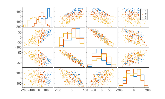
Visualize the generated data set using a set of scatter plots. Plot each pair of features on a separate axis and each class in a different color. The software also plots the outlines of the grouped histograms in the diagonal plots of the plot matrix.

gplotmatrix(X,[],T)

Define Network

Use the function createPFN, which is attached to this example as a supporting file, to create a PFN with 64 hidden units and six attention blocks. Create a PFN that can accept a maximum number of 20 features and predict a maximum of five classes.

numHiddenUnits = 64;
numAttnBlocks = 6;

maxNumFeatures = 20;
maxNumClasses = 5;

net = createPFN(maxNumFeatures,maxNumClasses,numHiddenUnits,numAttnBlocks);

Visualize Network

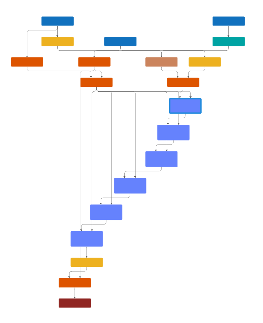
To view the network, use the Deep Network Designer app. The app displays the network layers and connections.

deepNetworkDesigner(net)

Visual represention of the network. The layers are represented by blocks with links between the blocks representing the connections. The color of the block represents the type.

The network treats each data set as a sequence, with the training data at the start of the sequence and the test data at the end. The training predictors, training targets, and test predictors feed into the network through sequence input layers.

The network uses a transformer architecture [3], made up of repeated attention blocks that are contained inside networkLayer objects. To view the contents of an attention block, double-click on the attn_1 layer in Deep Network Designer.

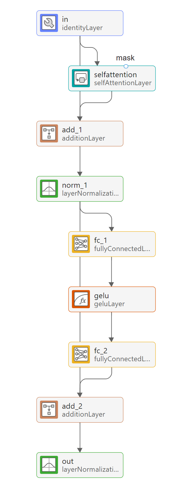
Visual representation of the layers and connections inside the attention block. The first layer is an identity layer and the final layer is a layer normalization layer. The block contains a self attention layer.

The attention layers in the network take a mask input, which has a value of 1 at indices corresponding to labeled observations and a value of 0 at indices corresponding to unlabeled observations. This ensures that the network does not compute attention scores between test data and training data when performing classification [2].

Define Model Loss Function

Create the function modelLoss, which computes the index cross-entropy loss between the network outputs and the test targets, along with its gradient.

function [loss,gradients] = modelLoss(net,XTrain,TTrain,XTest,TTest)

Y = forward(net,XTrain,TTrain,XTest);
loss = indexcrossentropy(Y,TTest);
gradients = dlgradient(loss,net.Learnables);

end

Accelerate the model loss function by using the dlaccelerate function. Clear any previously cached traces of the accelerated function by using the clearCache function.

accFun = dlaccelerate(@modelLoss);
clearCache(accFun);

Specify Training Options

Train with a mini-batch size of 64 for 10,000 iterations.

miniBatchSize = 64;
numIterations = 10000;

In each synthetic data set, generate 256 observations. Use half of these observations as labeled training data and the other half as unlabeled test data.

numObservationsPerDataSet = 256;
trainFraction = 0.5;
numTrainObservations = floor(trainFraction*numObservationsPerDataSet);

Train Prior-Data Fitted Network

Train the PFN using a custom training loop. The custom training loop allows you to generate and partition new data at every iteration, so you do not have to store the data. For each iteration:

Generate a new mini-batch of synthetic data by using the generateClassificationDataSet function.
Divide the mini-batch into training and test data.
Remove outliers and normalize the mini-batch using the training data statistics.
Pass the training predictors, training targets, and test predictors into the network.
Compute the model loss between the network outputs and the test targets, along with the gradient.
Update the learnable parameters of the network using gradient descent along the gradients of the loss function.

Training the model is a computationally expensive process. To save time while running this example, set doTraining to false to load a pretrained network. The pretrained network is approximately 0.6 MB in size. To train the network yourself, set doTraining to true.

doTraining = false;

Initialize the parameters for Adam optimization.

averageGrad = [];
averageSqGrad = [];

Define the function generateMiniBatch, which generates a mini-batch of synthetic data sets.

function [X,T] = generateMiniBatch(miniBatchSize,maxNumFeatures,maxNumClasses,numObservationsPerDataSet)

X = zeros(numObservationsPerDataSet,maxNumFeatures,miniBatchSize);
T = zeros(numObservationsPerDataSet,1,miniBatchSize);

for i = 1:miniBatchSize
    [X(:,:,i),T(:,:,i)] = generateClassificationDataSet(MaxNumFeatures=maxNumFeatures, ...
        MaxNumClasses=maxNumClasses, ...
        NumObservations=numObservationsPerDataSet);
end

end

Generating the synthetic data during training can take a long time. To speed up training, use the parfeval function to generate data in the background on a parallel pool while you compute the model loss and update the network. If a parallel pool is not available, then the parfeval function generates data serially. Using a parallel pool requires Parallel Computing Toolbox™.

if doTraining
    f(1:numIterations) = parallel.FevalFuture;

    for i = 1:numIterations
        f(i) = parfeval(@generateMiniBatch,2, ...
            miniBatchSize, ...
            maxNumFeatures, ...
            maxNumClasses, ...
            numObservationsPerDataSet);
    end
end

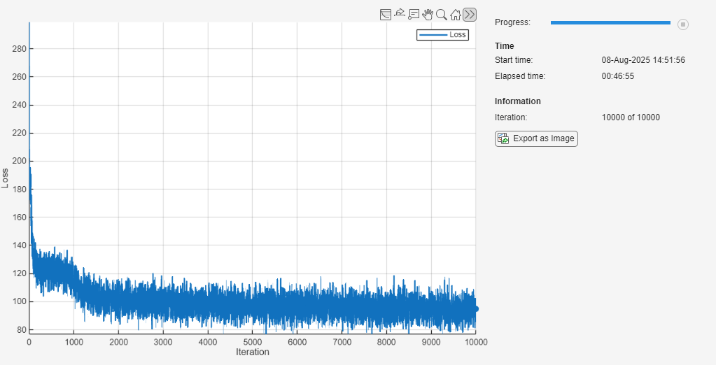
To track the model performance, use a trainingProgressMonitor object. Because the timer starts when you create the monitor object, create the object close to the training loop.

if doTraining
    monitor = trainingProgressMonitor( ...
        Metrics="Loss", ...
        Info="Iteration", ...
        XLabel="Iteration");
end

Train the network. The training loop uses a GPU if one is available. Using a GPU requires Parallel Computing Toolbox and a supported GPU device. For information on supported devices, see GPU Computing Requirements (Parallel Computing Toolbox).

if doTraining
    iteration = 0;

    while iteration < numIterations && ~monitor.Stop
        iteration = iteration + 1;

        % Fetch the generated data from the parallel pool.
        [~,X,T] = fetchNext(f);

        % Move the data to the GPU, if available.
        if canUseGPU
            X = gpuArray(X);
            T = gpuArray(T);
        end

        % Split predictors and targets into training and test sets.
        XTrain = X(1:numTrainObservations,:,:);
        TTrain = T(1:numTrainObservations,:,:);
        XTest = X(numTrainObservations+1:end,:,:);
        TTest = T(numTrainObservations+1:end,:,:);

        % Replace outliers with the median value of the training data
        % using the training statistics to determine outlier thresholds.
        [XTrain,~,lowerThreshold,upperThreshold,medianValue] = filloutliers(XTrain,"center",ThresholdFactor=10);
        isTestOutlier = ~isbetween(XTest,lowerThreshold,upperThreshold);
        XTest = XTest.*~isTestOutlier + medianValue.*isTestOutlier;

        % Normalize predictors based on training statistics.
        mu = mean(XTrain);
        sigma = std(XTrain);
        sigma(isapprox(sigma,0)) = 1;
        XTrain = (XTrain - mu) ./ sigma;
        XTest = (XTest - mu) ./ sigma;

        % Convert the data to dlarray objects so the loss function can be
        % traced.
        XTrain = dlarray(XTrain,"TCB");
        TTrain = dlarray(TTrain,"TCB");
        XTest = dlarray(XTest,"TCB");
        TTest = dlarray(TTest,"TCB");

        % Compute loss.
        [loss,gradients] = dlfeval(accFun,net,XTrain,TTrain,XTest,TTest);

        % Update model.
        [net,averageGrad,averageSqGrad] = adamupdate(net,gradients,averageGrad,averageSqGrad,iteration);

        % Record metrics.
        recordMetrics(monitor,iteration,Loss=loss);
        updateInfo(monitor,Iteration=iteration + " of " + numIterations);
        monitor.Progress = 100 * iteration/numIterations;
    end

    % Cancel any incomplete futures.
    cancel(f)
else
    load trainedPFN.mat
end

Training progress plot showing the loss at each iteration. The loss is decreasing as the number of iterations increases. On the right is a panel displaying the training progress, start time, elapsed time, and iteration number.

Classify New Data Sets

Test the network by classifying three real data sets that the network has not seen during training.

Define the function loadTestDataSet, which loads the three data sets and preprocesses them for testing. For more information about these data sets, see Statistics and Machine Learning Toolbox Example Data Sets (Statistics and Machine Learning Toolbox).

function [X,T,classes] = loadTestDataSet(dataSetName)

switch dataSetName
    case "iris"
        s = load("fisheriris.mat");
        X = s.meas;
        T = categorical(s.species);
    case "ionosphere"
        s = load("ionosphere.mat");
        X = s.X;
        T = categorical(s.Y);
    case "ovarian"
        s = load("ovariancancer.mat");
        X = s.predictors;
        T = s.targets;
end

classes = categories(T);

end

Load the test data set.

testDataSet = "ovarian";
[X,T,classes] = loadTestDataSet(testDataSet);
numFeatures = size(X,2);
numClasses = numel(classes);

The network has a fixed input size of maxNumFeatures. If the predictors have fewer features than this, then pad them with zeros so that their size is equal to maxNumFeatures and rescale them to keep their magnitude independent of the number of features.

numPredictorFeatures = size(X,2);

if numPredictorFeatures < maxNumFeatures
    X = padarray(X,[0 maxNumFeatures-numFeatures],"post");
    X = X * maxNumFeatures/numFeatures;
end

Partition the inputs randomly into a training and test set.

holdoutFraction = 0.5;
cvp = cvpartition(T,Holdout=holdoutFraction);
XTrain = X(cvp.training,:);
TTrain = T(cvp.training,:);
XTest = X(cvp.test,:);
TTest = T(cvp.test,:);

If the predictors have more features than maxNumFeatures, then use chi-square tests to select only the most important features, up to a total size of maxNumFeatures. To avoid exposing the model to information from the test data, use only the training data to rank the features.

if numPredictorFeatures > maxNumFeatures
    idx = fscchi2(XTrain,TTrain);
    selectedFeatures = idx(1:maxNumFeatures);
    XTrain = XTrain(:,selectedFeatures);
    XTest = XTest(:,selectedFeatures);
end

Replace outliers with the median of the training data. Use the statistics of the training data to determine outlier thresholds with a threshold factor of 10.

[XTrain,~,lowerThreshold,upperThreshold,medianValue] = filloutliers(XTrain,"center",ThresholdFactor=10);
isTestOutlier = ~isbetween(XTest,lowerThreshold,upperThreshold);
XTest = XTest.*~isTestOutlier + medianValue.*isTestOutlier;

Use the statistics of the training data to normalize the predictors so that they have zero mean and unit variance. Do not rescale features with zero variance.

mu = mean(XTrain);
sigma = std(XTrain);
sigma(isapprox(sigma,0)) = 1;
XTrain = (XTrain - mu) ./ sigma;
XTest = (XTest - mu) ./ sigma;

Use the trained network to classify the new data set. The trained network learns from the training data and classifies the test data in a single inference pass, without retraining. This method is called in-context learning.

scores = predict(net,XTrain,double(TTrain),XTest);
scores = scores(:,1:numClasses);
YTest = scores2label(scores,classes);

Compute the accuracy of the classifier.

accuracy = sum(YTest==TTest) / numel(TTest)

accuracy = 
0.8981

Visualize the performance of the classifier using a confusion chart.

figure
confusionchart(TTest,YTest)

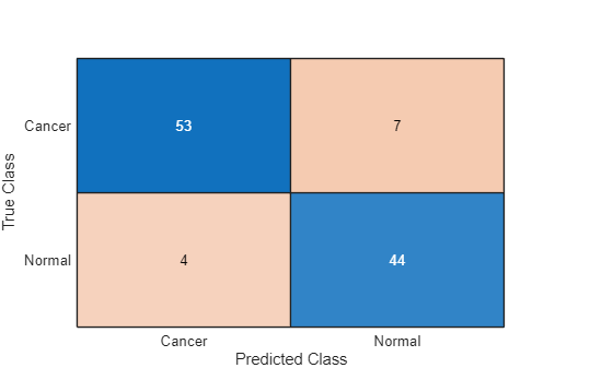
Figure contains an object of type ConfusionMatrixChart.

Despite only being trained on synthetic data, the network performs well when classifying real data across different domains.

Synthetic Data Generation Process

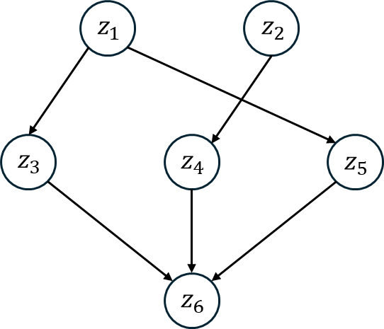
The function generateClassificationDataSet, which is attached to this example as a supporting file, generates a synthetic set of labeled data for classification. To generate realistic tabular data, the function uses an algorithm based on structural causal models (SCMs). Structural causal models represent data variables as nodes in a directed acyclic graph (DAG), with an edge between two nodes indicating that one causes the other. Values at connected nodes are linked by a structural equation, which this example assumes is of the form

$y = f (w x + ϵ),$

where

$x$ and $y$ are variables, with $x$ causing $y$ .
$w$ is the weight of the edge between the two nodes, a constant.
$ϵ$ is random noise drawn from a normal distribution.
$f$ is a nonlinear activation function.

This figure shows a diagram of an SCM with six nodes. In this model, $z_{1}$ is a direct cause of $z_{3}$ and $z_{5},$ $z_{2}$ is a direct cause of $z_{4},$ and $z_{3},$ $z_{4},$ and $z_{5}$ are all direct causes of $z_{6}$ .

A diagram of a structural causal model with six nodes, z_1 to z_6. z_1 is a direct cause of z_3 and z_5. z_2 is a direct cause of z_4. z_3, z_4 and z_5 are all direct causes of z_6. There are no other causal relationships in the graph.

The function generates a data set using the following algorithm [2]. Steps 1-5 define a sparse multilayer perceptron with random weights and a random bias that changes with every forward pass.

Sample a random number of layers and a random number of nodes per layer. Denote the value at a node with index $i$ by $z_{i} .$
Sample random weight matrices $W_{ij}$ for each layer.
Set values from the weight matrices to zero either randomly, or to make the matrices block diagonal with a random number of blocks. This step defines a sparsely connected DAG, with each element of $W_{ij}$ indicating the weight of an edge.
Sample random noise values $ϵ_{i}$ to be added at each node.
Sample a random activation function $f$ from a choice of activation functions.
Sample random initial data with a random number of input variables and pass it through the neural network, computing the outputs after each activation function.
Choose a random set of output values to be the predictors in the data set.
Choose a single output to be the target, either randomly or from the last layer in the network.
Discretize the target variable to a random number of classes, with bin boundaries sampled randomly from the outputs of the target node.

The algorithm draws several random variables, each from a different distribution. The algorithm uses the same distributions as those in [2].

You can view using synthetic data to train the PFN as assuming that real data follows the distribution encoded in the data generation algorithm. In Bayesian statistics, this assumed distribution is known as a prior.

References

[1] Müller, Samuel et al. "Transformers Can Do Bayesian Inference." Proceedings of the International Conference on Learning Representations (ICLR'22), 2022. https://openreview.net/forum?id=KSugKcbNf9.

[2] Hollmann, Noah, et al. "TabPFN: A Transformer That Solves Small Tabular Classification Problems in a Second." Proceedings of the International Conference on Learning Representations (ICLR'23), 2023 https://openreview.net/forum?id=cp5PvcI6w8_.

[3] Vaswani, A., N. et al. "Attention Is All You Need." Advances in Neural Information Processing Systems 30, 2017. https://proceedings.neurips.cc/paper_files/paper/2017/file/3f5ee243547dee91fbd053c1c4a845aa-Paper.pdf.