Generate C Code for Inference Models Used in Transmission System Fault Detection
R2026bThis example shows how to generate production C code for detecting sensor drift and shaft wear in an automotive transmission system. Use software-in-the-loop (SIL) simulation to verify that the generated code satisfies the requirements outlined in Code Generation Inference Requirements.
Load MATLAB Models and Data
First, load the sensor drift classifier SDClassifier and the shaft wear classifier SWClassifier into the MATLAB workspace from the faultDetectionModels.mat file. For more information on how to create these classifiers, see Perform Feature Selection and Model Training for Transmission System Fault Detection.
load("faultDetectionModels.mat","SDClassifier","SWClassifier");
Load the signal data for the eight fault and failure scenarios described in Fault and Failure Scenarios.
supportFileNames = ["faultScenario1","faultScenario2","faultScenario3","faultScenario4", ...
    "faultScenario5","faultScenario6","faultScenario7","faultScenario8"];
scenarioVarNames = ["dataTable_s1","dataTable_s2","dataTable_s3","dataTable_s4", ...
    "dataTable_s5","dataTable_s6","dataTable_s7","dataTable_s8"];

signalData = table;
for k = 1:numel(supportFileNames)
    d = load(matlab.internal.examples.downloadSupportFile("nnet", ...
        "data/transmissionfaults/" + supportFileNames(k) + ".mat"));
    scenarioTable = d.(scenarioVarNames(k));
    scenarioTable.ScenarioID = repmat(k,height(scenarioTable),1);
    signalData = [signalData; scenarioTable];
end
Use 30% of the signal data for verification of the model behavior after code generation.
rng(1,"twister");
cv = cvpartition(signalData.ScenarioID,HoldOut=0.3);
signalTestData = signalData(cv.test,:);
numObs = height(signalTestData)
numObs = 552
signalTestData contains the test set observations.
Generate Predictions in MATLAB
Generate test set predictions in MATLAB, for later comparison. For each fault type, first extract the features from signalTestData that were used to train the classifier. Then, use the predict function to compute the predicted labels.
sdPredMatlab = zeros(numObs,1);
swPredMatlab = zeros(numObs,1);

for i = 1:numObs
    v = signalTestData.Vibration{i}.Data;
    sdFeatures = [max(v) peak2rms(v)];
    sdPredMatlab(i) = predict(SDClassifier,sdFeatures);

    tpSec = seconds(signalTestData.TachoPulses{i});
    nPulses = numel(tpSec);
    if nPulses > 1
        dtPulse = diff(tpSec);
        rpmInst = 60 ./ dtPulse;
        rpmIQR = iqr(rpmInst);
        rpmStd = std(rpmInst,0,"omitnan");
    else
        rpmIQR = NaN;
        rpmStd = NaN;
    end
    swFeatures = [rpmIQR rpmStd];
    swPredMatlab(i) = predict(SWClassifier,swFeatures);
end
sdPredMatlab contains the test set predicted labels returned by the sensor drift model SDClassifier, and swPredMatlab contains the test set predicted labels returned by the shaft wear model SWClassifier.
Configure Simulink Model for Time Profiling in SIL Mode
Open the Simulink model AIFaultDetectorComponent, which contains two fault detection subsystems: one for detecting sensor drift and one for detecting shaft wear. The Sensor Drift Fault Detector subsystem corresponds to the SDClassifier model in MATLAB, and the Shaft Wear Fault Detector subsystem corresponds to the SWClassifier model in MATLAB.
open_system("AIFaultDetectorComponent");Before you can generate code and run the Simulink model in SIL mode, follow these steps to configure the model:
Open the Configuration Parameters dialog box. In the Simulink Editor, on the Modeling tab, click Model Settings.
In the Code Generation pane, under Target selection, specify
ert.tlcas the System target file value.In the Code Generation > Verification pane, under Code execution time profiling, select the Measure task execution time check box.
For the function execution times, select
Coarse (referenced models and subsystems only)from the Measure function execution times list. This option allows you to analyze generated function code for the main model components.In the Workspace variable field, specify the variable name as
executionProfile. When you run the simulation, the software generates a variable with this name in the MATLAB base workspace. The variable, an object of typecoder.profile.ExecutionTime, contains the execution time measurements.Select
Metrics onlyfrom the Save options list. This option helps reduce bandwidth usage for the communication channel between Simulink and the target application.In the Data Import/Export pane, under Save to workspace or file, select the Single simulation output check box and specify the variable name as
out. During simulation, the software creates theexecutionProfilevariable in theoutvariable (Simulink.SimulationOutputobject).In the Hardware Implementation pane, select the type of hardware to use to implement the system represented by the model. This example uses the default value
x86–64 (Windows64).Click OK.
To generate function execution data, you must insert measurement probes into the generated code. The software can insert measurement probes for an atomic subsystem only if you set the Function packaging field (on the Code Generation tab of the Block Parameters dialog box) to either Nonreusable function or Reusable function. To enable granular execution profiling for each predict block, place the prediction blocks inside a subsystem. For each predict block that is not a MATLAB Function block:
Right-click the block, and select Create Subsystem from Selection > Atomic Subsystem.
Rename the subsystem to have the same name as the corresponding MATLAB classifier.
For each subsystem block and MATLAB Function block:
Open the Block Parameters dialog box. Right-click the block, and click the Block Parameters icon in the Parameters row.
On the Main tab, select the Treat as atomic unit check box.
On the Code Generation tab, change Function packaging to Nonreusable function. Then click OK.
The prediction implementations that use MATLAB Function blocks require support for variable signals to be enabled for code generation. To enable code generation support:
Open the Configuration Parameters dialog box. In the Simulink Editor, on the Modeling tab, click Model Settings.
In the Code Generation > Interface pane, under Software environment, select the variable-size signals check box. Then click OK.
Close the model.
close_system("AIFaultDetectorComponent");Generate Predictions from Simulink Model in SIL Mode
Open the Simulink model AIFDProfiling, which corresponds to the AIFaultDetectorComponent model, already configured for SIL profiling.
modelName = "AIFDProfiling";
open_system(modelName);
Use the model to generate predictions in SIL mode.
Prepare Simulink Input Data
Before generating test set predictions in Simulink, prepare the data. Convert the signal test data into numeric arrays. Then, create grouped simulation data using a Simulink.SimulationData.Dataset object. Each time step provides one full observation window to the fault detection subsystems.
Ts = 0.001;
t = (0:numObs-1)' * Ts;

vibMatrix = zeros(numObs,30000);
tpMatrix = zeros(numObs,30);
nPulsesVec = zeros(numObs,1);

for i = 1:numObs
    vibMatrix(i,:) = signalTestData.Vibration{i}.Data';
    tp = seconds(signalTestData.TachoPulses{i});
    nPulsesVec(i) = numel(tp);
    tpMatrix(i, 1:nPulsesVec(i)) = tp';
end

vibIn = timeseries(vibMatrix,t,Name="winVibration");
tpIn = timeseries(tpMatrix,t,Name="winTachoPulses");
nIn = timeseries(int32(nPulsesVec),t,Name="nPulses");

ds = Simulink.SimulationData.Dataset;
ds = ds.addElement(vibIn,"winVibration");
ds = ds.addElement(tpIn,"winTachoPulses");
ds = ds.addElement(nIn,"nPulses");
Generate Code and Run SIL Simulation
Generate code and run the SIL simulation with the test data set stored in ds. The software returns the generated code and build artifacts within the slprj folder in the current directory.
set_param(modelName,SimulationMode="software-in-the-loop");
set_param(modelName,RTWVerbose="off");
simIn = Simulink.SimulationInput(modelName);
simIn = simIn.setExternalInput(ds);
out = sim(simIn);
### Searching for referenced models in model 'AIFDProfiling'.
### Total of 1 models to build.
### Starting top model code generation target build for: AIFDProfiling
### Successful completion of build procedure for: AIFDProfiling

Build Summary

Top model targets:

Model          Build Reason                             Status                        Build Duration
====================================================================================================
AIFDProfiling  Target (AIFDProfiling.c) did not exist.  Code generated and compiled.  0h 0m 47.592s

1 of 1 models built (0 models already up to date)
Build duration: 0h 0m 49.217s
### Preparing to start SIL simulation ...
Building with 'MinGW64 Compiler (C)'.
MEX completed successfully.
### Starting SIL simulation for component: AIFDProfiling
### Application stopped
### Stopping SIL simulation for component: AIFDProfiling
Extract Generated Predictions
Extract the generated predictions from the Simulink.SimulationOutput object out. Limit the number of observations to numObs, in case extra sample predictions are made.
yout = out.yout;
sdPredSIL = yout.getElement(1).Values.Data;
sdPredSIL = sdPredSIL(1:numObs);

swPredSIL = yout.getElement(2).Values.Data;
swPredSIL = swPredSIL(1:numObs);
sdPredSIL contains the test set predicted labels returned by the Sensor Drift Fault Detector subsystem, and swPredSIL contains the test set predicted labels returned by the Shaft Wear Fault Detector subsystem.
Extract Execution Times
Launch the SIL/PIL app from the Simulink toolstrip. In the Results section of the SIL/PIL tab, click Compare Runs and select Code Profile Analyzer. In the Code Profile Analyzer window, under the Analysis section, select Function Execution. Navigate to the end of the list of blocks to locate the prediction blocks, and compare their execution times. Note that execution times can vary across runs.
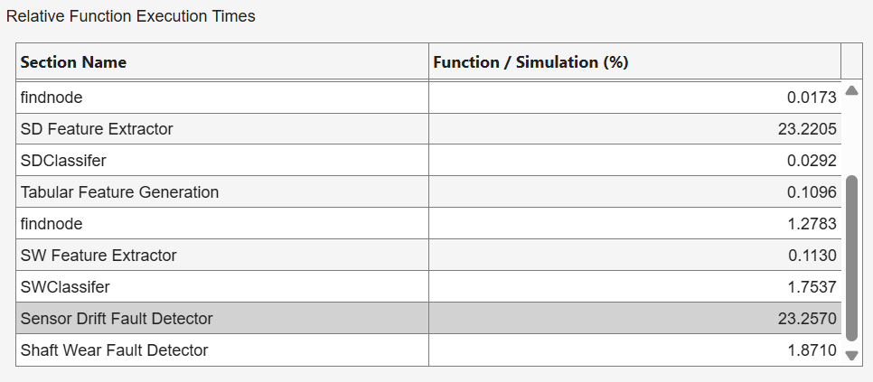
The profiling report indicates that the Sensor Drift Fault Detector subsystem in much slower than the Shaft Wear Fault Detector subsystem, despite using a simpler decision tree model. This result indicates that the feature extraction process in sensor drift detection is much more time-consuming than the shaft wear feature extraction process.
Programmatically extract the execution time information from out.
executionProfileLog = out.executionProfile;
faultDetectorsProfileLog = executionProfileLog.Sections([12 13]);
{faultDetectorsProfileLog.Name}'
ans = 2×1 cell array
{'Sensor Drift Fault Detector'}
{'Shaft Wear Fault Detector' }
timerTicksPerSecond = executionProfileLog.TimerTicksPerSecond;
sdTotalExecutionTimeInTicks = ...
    double(faultDetectorsProfileLog(1).TotalExecutionTimeInTicks);
swTotalExecutionTimeInTicks = ...
    double(faultDetectorsProfileLog(2).TotalExecutionTimeInTicks);
sdInferenceTimeSIL = sdTotalExecutionTimeInTicks/timerTicksPerSecond
sdInferenceTimeSIL =
0.1749
swInferenceTimeSIL = swTotalExecutionTimeInTicks/timerTicksPerSecond
swInferenceTimeSIL =
0.0182
sdInferenceTimeSIL is the time (in seconds) used to generate test set predictions for sensor drift detection. Similarly, swInferenceTimeSIL is the time (in seconds) used to generated test set predictions for shaft wear detection.
These inference speed results differ from those in Import and Verify Models in Simulink for Transmission System Fault Detection, where simulations are run in normal mode. In normal mode, the inference speed for shaft wear detection is slower than the inference speed for sensor drift detection because the underlying ensemble classifier's many tree evaluations are expensive. In SIL mode, the compiled C code makes model inference fast for both classifiers, and the bottleneck shifts to feature extraction.
Verify Code Generation Inference Requirements
Verify that the compiled C implementation in SIL mode satisfies the requirements described in Code Generation Inference Requirements. In particular, verify that the test set predictions returned by the generated code match the test set predictions in MATLAB. Also verify that the predictions are generated sufficiently quickly. Use the helper function helperVerifyRequirements to summarize the results in a table.
verificationTable = helperVerifyRequirements( ...
    sdPredMatlab,sdPredSIL,swPredMatlab,swPredSIL, ...
    sdInferenceTimeSIL,swInferenceTimeSIL)
verificationTable = 4×4 table
        RequirementID                                  Description                               Metric      Result
    ______________________    ______________________________________________________________    ________    ________

    "SD_MODEL_EQUIVALENCE"    "Sensor drift SIL predictions match MATLAB (552 observations)"         100    "PASSED"
    "SW_MODEL_EQUIVALENCE"    "Shaft wear SIL predictions match MATLAB (552 observations)"           100    "PASSED"
    "SD_INFERENCE_SPEED"      "Sensor drift SIL inference < 1 sec"                               0.17495    "PASSED"
    "SW_INFERENCE_SPEED"      "Shaft wear SIL inference < 1 sec"                                0.018218    "PASSED"

	Get insights using Copilot
The verification table shows that the generated code meets all requirements.
Helper Function
The helperVerifyRequirements function determines whether the requirements described in Code Generation Inference Requirements are met, given the MATLAB test set predictions for sensor drift and shaft wear (sdPredMatlab and swPredMatlab, respectively), the SIL test set predictions for sensor drift and shaft wear (sdPredSIL and swPredSIL, respectively), and the SIL inference times for sensor drift and shaft wear (sdInferenceTimeSIL and swInferenceTimeSIL, respectively). The function returns a table (verificationTable) with the results.
function verificationTable = helperVerifyRequirements( ...
    sdPredMatlab,sdPredSIL,swPredMatlab,swPredSIL, ...
    sdInferenceTimeSIL,swInferenceTimeSIL)

nReqs = 4;
RequirementID = strings(nReqs,1);
Description = strings(nReqs,1);
Metric = zeros(nReqs,1);
Result = strings(nReqs,1);

numObs = height(sdPredMatlab);
sdMatch = isequal(sdPredMatlab,sdPredSIL);
RequirementID(1) = "SD_MODEL_EQUIVALENCE";
Description(1) = sprintf("Sensor drift SIL predictions match MATLAB (%d observations)",numObs);
Metric(1) = sum(sdPredMatlab == sdPredSIL) / numObs*100;
if sdMatch
    Result(1) = "PASSED";
else
    Result(1) = "FAILED";
end

swMatch = isequal(swPredMatlab,swPredSIL);
RequirementID(2) = "SW_MODEL_EQUIVALENCE";
Description(2) = sprintf("Shaft wear SIL predictions match MATLAB (%d observations)",numObs);
Metric(2) = sum(swPredMatlab == swPredSIL) / numObs*100;
if swMatch
    Result(2) = "PASSED";
else
    Result(2) = "FAILED";
end

RequirementID(3) = "SD_INFERENCE_SPEED";
Description(3) = sprintf("Sensor drift SIL inference < 1 sec");
Metric(3) = sdInferenceTimeSIL;
if Metric(3) < 1
    Result(3) = "PASSED";
else
    Result(3) = "FAILED";
end

RequirementID(4) = "SW_INFERENCE_SPEED";
Description(4) = sprintf("Shaft wear SIL inference < 1 sec");
Metric(4) = swInferenceTimeSIL;
if Metric(4) < 1
    Result(4) = "PASSED";
else
    Result(4) = "FAILED";
end

verificationTable = table(RequirementID,Description,Metric,Result);
end
See Also
Simulink.SimulationData.Datasetsim (Simulink) | SIL/PIL Manager (Embedded Coder) | predict (Statistics and Machine Learning Toolbox) | predict (Statistics and Machine Learning Toolbox)

