Create Reference Model Controller with MATLAB Script
So far, this topic has described the training procedures for several specific dynamic network architectures. However, any network that can be created in the toolbox can be trained using the training functions described in Multilayer Shallow Neural Networks and Backpropagation Training so long as the components of the network are differentiable. This section gives an example of how to create and train a custom architecture. The custom architecture you will use is the model reference adaptive control (MRAC) system that is described in detail in Design Model-Reference Neural Controller in Simulink.
As you can see in Design Model-Reference Neural Controller in Simulink, the model reference control architecture has two subnetworks. One subnetwork is the model of the plant that you want to control. The other subnetwork is the controller. You will begin by training a NARX network that will become the plant model subnetwork. For this example, you will use the robot arm to represent the plant, as described in Design Model-Reference Neural Controller in Simulink. The following code will load data collected from the robot arm and create and train a NARX network. For this simple problem, you do not need to preprocess the data, and all of the data can be used for training, so no data division is needed.
Note
To design a model reference adaptive controller, you can also use the Model Reference Adaptive Control (Simulink Control Design) Simulink® block.
This workflow is recommended because of these advantages:
Simplifies the controller design.
Requires only an initial guess of the plant model dynamics.
Automatically characterizes disturbances and model uncertainties such as single hidden layer neural networks. The block then updates controller parameters in real-time to cancel out these disturbances and uncertainties in the controlled system, removing the need for manual retuning. For more information on using single hidden layer neural networks, see Disturbance and Uncertainty Model (Simulink Control Design).
Supports code generation.
For an example showing how to use these tools, see Quadrotor Control Using Model Reference Adaptive Control (Simulink Control Design).
[u,y] = robotarm_dataset;
d1 = [1:2];
d2 = [1:2];
S1 = 5;
narx_net = narxnet(d1,d2,S1);
narx_net.divideFcn = '';
narx_net.inputs{1}.processFcns = {};
narx_net.inputs{2}.processFcns = {};
narx_net.outputs{2}.processFcns = {};
narx_net.trainParam.min_grad = 1e-10;
[p,Pi,Ai,t] = preparets(narx_net,u,{},y);
narx_net = train(narx_net,p,t,Pi);
narx_net_closed = closeloop(narx_net);
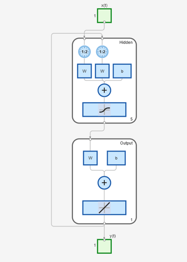
view(narx_net_closed)


The resulting network is shown in the figure.
Now that the NARX plant model is trained, you can create the total MRAC system and insert the NARX model inside. Begin with a feedforward network, and then add the feedback connections. Also, turn off learning in the plant model subnetwork, since it has already been trained. The next stage of training will train only the controller subnetwork.
mrac_net = feedforwardnet([S1 1 S1]);
mrac_net.layerConnect = [0 1 0 1;1 0 0 0;0 1 0 1;0 0 1 0];
mrac_net.outputs{4}.feedbackMode = 'closed';
mrac_net.layers{2}.transferFcn = 'purelin';
mrac_net.layerWeights{3,4}.delays = 1:2;
mrac_net.layerWeights{3,2}.delays = 1:2;
mrac_net.layerWeights{3,2}.learn = 0;
mrac_net.layerWeights{3,4}.learn = 0;
mrac_net.layerWeights{4,3}.learn = 0;
mrac_net.biases{3}.learn = 0;
mrac_net.biases{4}.learn = 0;
The following code turns off data division and preprocessing, which are not needed for this example problem. It also sets the delays needed for certain layers and names the network.
mrac_net.divideFcn = '';
mrac_net.inputs{1}.processFcns = {};
mrac_net.outputs{4}.processFcns = {};
mrac_net.name = 'Model Reference Adaptive Control Network';
mrac_net.layerWeights{1,2}.delays = 1:2;
mrac_net.layerWeights{1,4}.delays = 1:2;
mrac_net.inputWeights{1}.delays = 1:2;
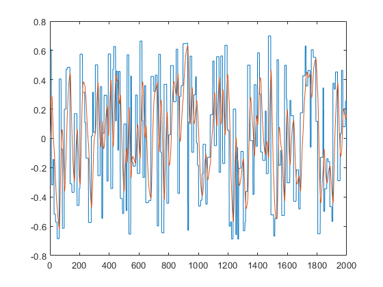
To configure the network, you need some sample training data. The following code loads and plots the training data, and configures the network:
[refin,refout] = refmodel_dataset;
ind = 1:length(refin);
plot(ind,cell2mat(refin),ind,cell2mat(refout))
mrac_net = configure(mrac_net,refin,refout);

You want the closed-loop MRAC system to respond in the same way as the reference model that was used to generate this data. (See Use the Model Reference Controller Block for a description of the reference model.)
Now insert the weights from the trained plant model network into the appropriate location of the MRAC system.
mrac_net.LW{3,2} = narx_net_closed.IW{1};
mrac_net.LW{3,4} = narx_net_closed.LW{1,2};
mrac_net.b{3} = narx_net_closed.b{1};
mrac_net.LW{4,3} = narx_net_closed.LW{2,1};
mrac_net.b{4} = narx_net_closed.b{2};
You can set the output weights of the controller network to zero, which will give the plant an initial input of zero.
mrac_net.LW{2,1} = zeros(size(mrac_net.LW{2,1}));
mrac_net.b{2} = 0;
You can also associate any plots and training function that you want to the network.
mrac_net.plotFcns = {'plotperform','plottrainstate',...
    'ploterrhist','plotregression','plotresponse'};
mrac_net.trainFcn = 'trainlm';
The final MRAC network can be viewed with the following command:
view(mrac_net)

Layer 3 and layer 4 (output) make up the plant model subnetwork. Layer 1 and layer 2 make up the controller.
You can now prepare the training data and train the network.
[x_tot,xi_tot,ai_tot,t_tot] = ...
    preparets(mrac_net,refin,{},refout);
mrac_net.trainParam.epochs = 50;
mrac_net.trainParam.min_grad = 1e-10;
[mrac_net,tr] = train(mrac_net,x_tot,t_tot,xi_tot,ai_tot);

Note
Notice that you are using the trainlm training function here, but any of the
training functions discussed in Multilayer Shallow Neural Networks and Backpropagation Training could be used as well. Any network that
you can create in the toolbox can be trained with any of those training functions. The only
limitation is that all of the parts of the network must be differentiable.
You will find that the training of the MRAC system takes much longer that the training of the NARX plant model. This is because the network is recurrent and dynamic backpropagation must be used. This is determined automatically by the toolbox software and does not require any user intervention. There are several implementations of dynamic backpropagation (see [DeHa07]), and the toolbox software automatically determines the most efficient one for the selected network architecture and training algorithm.
After the network has been trained, you can test the operation by applying a test input to the MRAC network. The following code creates a test data set which is a series of steps of random height and width, and applies it to the trained MRAC network.
numBuildings = 10;
numDataPoints = 100;

buildingHeights = (rand(numBuildings,1)*2) - 1;
skylineData = zeros(1,numBuildings*numDataPoints);

for i = 1:numBuildings
    startIndex = (i - 1)*numDataPoints + 1;
    endIndex = i*numDataPoints;
    skylineData(startIndex:endIndex) = buildingHeights(i);
end

testin = skylineData;
testinseq = con2seq(testin);
testoutseq = mrac_net(testinseq);
testout = cell2mat(testoutseq);
figure
plot([testin' testout'])

From the figure, you can see that the plant model output does follow the reference input with the correct critically damped response, even though the input sequence was not the same as the input sequence in the training data. The steady state response is not perfect for each step, but this could be improved with a larger training set and perhaps more hidden neurons.
The purpose of this example was to show that you can create your own custom dynamic network and train it using the standard toolbox training functions without any modifications. Any network that you can create in the toolbox can be trained with the standard training functions, as long as each component of the network has a defined derivative.
It should be noted that recurrent networks are generally more difficult to train than feedforward networks. See [HDH09] for some discussion of these training difficulties.