Deep Network Quantizer

Quantize a deep neural network to 8-bit scaled integer data types

Description

Use the Deep Network Quantizer app to reduce the memory requirement of a deep neural network by quantizing weights, biases, and activations of convolution layers to 8-bit scaled integer data types. Using this app you can:

• Visualize the dynamic ranges of convolution layers in a deep neural network.

• Select individual network layers to quantize.

• Assess the performance of a quantized network.

• Generate GPU code to deploy the quantized network using GPU Coder™.

• Generate HDL code to deploy the quantized network to an FPGA using Deep Learning HDL Toolbox™.

• Generate C++ code to deploy the quantized network to an ARM Cortex-A microcontroller using MATLAB^® Coder™.

The Deep Learning Toolbox™ Model Quantization Library support package is a free add-on that you can download using the Add-On Explorer. Alternatively, see Deep Learning Toolbox Model Quantization Library. To learn about the products required to quantize and deploy the deep learning network to a GPU, FPGA, or CPU environment, see Quantization Workflow Prerequisites.

×

Open the Deep Network Quantizer App

• MATLAB command prompt: Enter deepNetworkQuantizer.

• MATLAB toolstrip: On the Apps tab, under Machine Learning and Deep Learning, click the app icon.

Examples

Quantize a Network for GPU Deployment

To explore the behavior of a neural network with quantized convolution layers, use the Deep Network Quantizer app. This example quantizes the learnable parameters of the convolution layers of the squeezenet neural network after retraining the network to classify new images according to the Train Deep Learning Network to Classify New Images example.

This example uses a DAG network with the GPU execution environment.

Load the network to quantize into the base workspace.

load squeezenetmerch
net

net = 
  DAGNetwork with properties:

         Layers: [68×1 nnet.cnn.layer.Layer]
    Connections: [75×2 table]
     InputNames: {'data'}
    OutputNames: {'new_classoutput'}

Define calibration and validation data.

The app uses calibration data to exercise the network and collect the dynamic ranges of the weights and biases in the convolution and fully connected layers of the network and the dynamic ranges of the activations in all layers of the network. For the best quantization results, the calibration data must be representative of inputs to the network.

The app uses the validation data to test the network after quantization to understand the effects of the limited range and precision of the quantized learnable parameters of the convolution layers in the network.

In this example, use the images in the MerchData data set. Define an augmentedImageDatastore object to resize the data for the network. Then, split the data into calibration and validation data sets.

unzip('MerchData.zip');
imds = imageDatastore('MerchData', ...
    'IncludeSubfolders',true, ...
    'LabelSource','foldernames');
[calData, valData] = splitEachLabel(imds, 0.7, 'randomized');
aug_calData = augmentedImageDatastore([227 227], calData);
aug_valData = augmentedImageDatastore([227 227], valData);

At the MATLAB command prompt, open the app.

deepNetworkQuantizer

In the app, click New and select Quantize a network.

The app verifies your execution environment. For more information, see Quantization Workflow Prerequisites.

In the dialog, select the execution environment and the network to quantize from the base workspace. For this example, select a GPU execution environment and the DAG network, net.

The app displays the layer graph of the selected network.

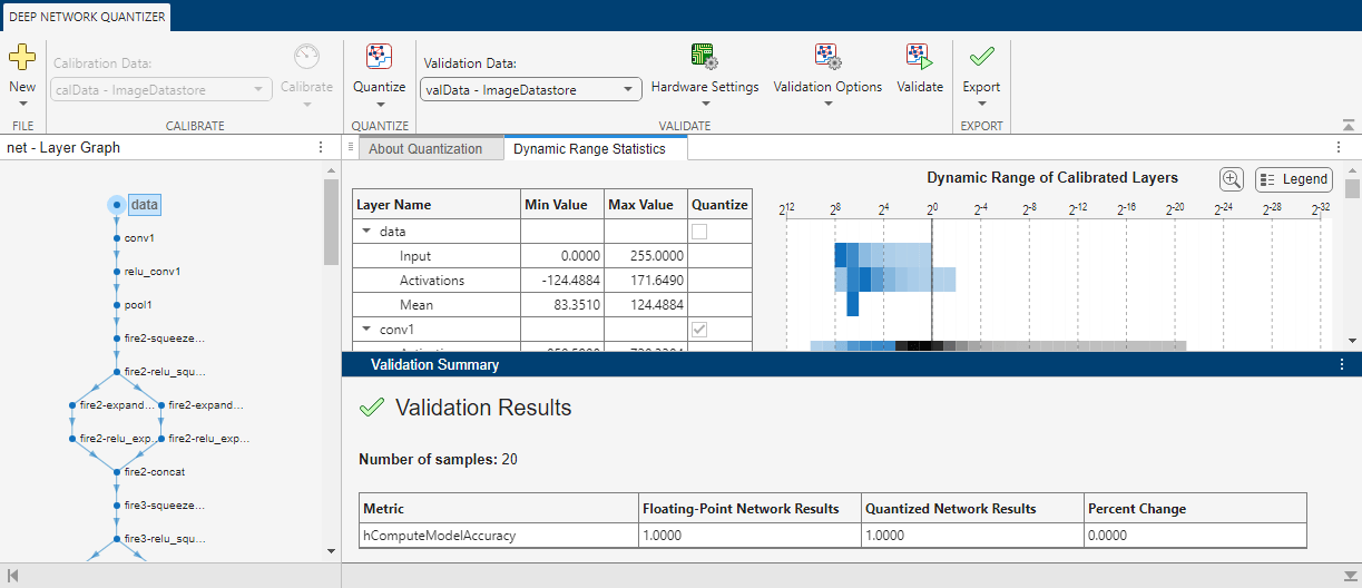
In the Calibrate section of the toolstrip, under Calibration Data, select the augmentedImageDatastore object from the base workspace containing the calibration data, calData.

Click Calibrate.

The Deep Network Quantizer uses the calibration data to exercise the network and collect range information for the learnable parameters in the network layers.

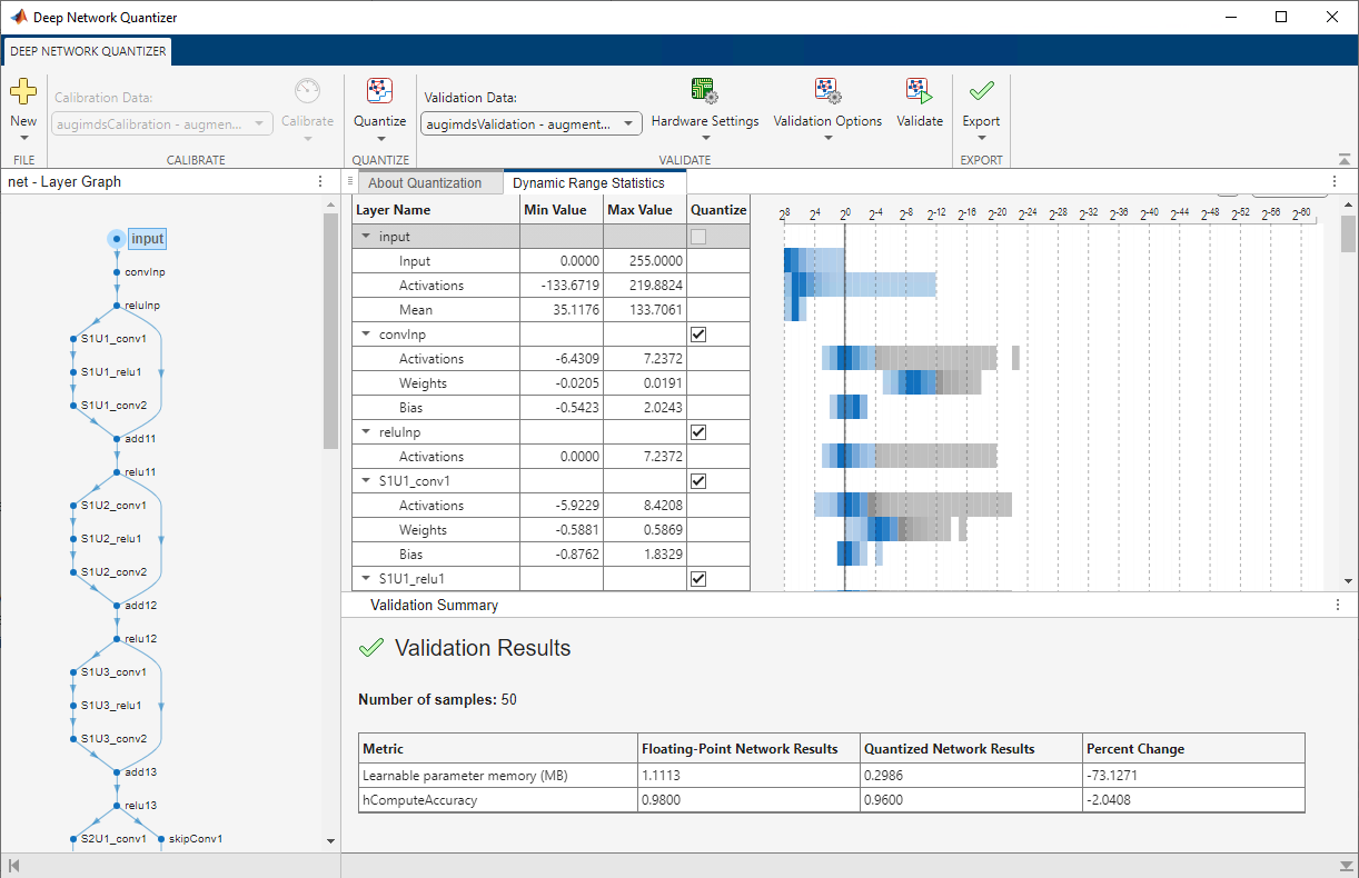
When the calibration is complete, the app displays a table containing the weights and biases in the convolution and fully connected layers of the network and the dynamic ranges of the activations in all layers of the network and their minimum and maximum values during the calibration. To the right of the table, the app displays histograms of the dynamic ranges of the parameters. The gray regions of the histograms indicate data that cannot be represented by the quantized representation. For more information on how to interpret these histograms, see Quantization of Deep Neural Networks.

In the Quantize column of the table, indicate whether to quantize the learnable parameters in the layer. Layers that are not convolution layers cannot be quantized, and therefore cannot be selected. Layers that are not quantized remain in single-precision after quantization.

In the Validate section of the toolstrip, under Validation Data, select the augmentedImageDatastore object from the base workspace containing the validation data, aug_valData.

In the Validate section of the toolstrip, under Quantization Options, select the Default metric function.

Click Quantize and Validate.

The Deep Network Quantizer quantizes the weights, activations, and biases of convolution layers in the network to scaled 8-bit integer data types and uses the validation data to exercise the network. The app determines a default metric function to use for the validation based on the type of network that is being quantized. For a classification network, the app uses Top-1 Accuracy.

When the validation is complete, the app displays the results of the validation, including:

• Metric function used for validation

• Result of the metric function before and after quantization

• Memory requirement of the network before and after quantization (MB)

If you want to use a different metric function for validation, for example to use the Top-5 accuracy metric function instead of the default Top-1 accuracy metric function, you can define a custom metric function. Save this function in a local file.

function accuracy = hComputeModelAccuracy(predictionScores, net, dataStore)
%% Computes model-level accuracy statistics
    
    % Load ground truth
    tmp = readall(dataStore);
    groundTruth = tmp.response;
    
    % Compare with predicted label with actual ground truth 
    predictionError = {};
    for idx=1:numel(groundTruth)
        [~, idy] = max(predictionScores(idx,:)); 
        yActual = net.Layers(end).Classes(idy);
        predictionError{end+1} = (yActual == groundTruth(idx)); %#ok
    end
    
    % Sum all prediction errors.
    predictionError = [predictionError{:}];
    accuracy = sum(predictionError)/numel(predictionError);
end

To revalidate the network using this custom metric function, under Quantization Options, enter the name of the custom metric function, hComputeModelAccuracy. Select Add to add hComputeModelAccuracy to the list of metric functions available in the app. Select hComputeModelAccuracy as the metric function to use.

The custom metric function must be on the path. If the metric function is not on the path, this step will produce an error.

Click Quantize and Validate.

The app quantizes the network and displays the validation results for the custom metric function.

The app displays only scalar values in the validation results table. To view the validation results for a custom metric function with non-scalar output, export the dlquantizer object as described below, then validate using the validate function at the MATLAB command window.

After quantizing and validating the network, you can choose to export the quantized network.

Click the Export button. In the drop down, select Export Quantizer to create a dlquantizer object in the base workspace. To open the GPU Coder app and generate GPU code from the quantized neural network, select Generate Code. Generating GPU code requires a GPU Coder license.

If the performance of the quantized network is not satisfactory, you can choose to not quantize some layers by deselecting the layer in the table. To see the effects, click Quantize and Validate again.

Import a dlquantizer Object into the Deep Network Quantizer App

This example shows you how to import a dlquantizer object from the base workspace into the Deep Network Quantizer app. This allows you to begin quantization of a deep neural network using the command line or the app, and resume your work later in the app.

Open the Deep Network Quantizer app.

deepNetworkQuantizer

In the app, click New and select Import dlquantizer object.

In the dialog, select the dlquantizer object to import from the base workspace. For this example, use quantObj that you create in the above example Quantize a Neural Network for GPU Target.

The app imports any data contained in the dlquantizer object that was collected at the command line. This data can include the network to quantize, calibration data, validation data, and calibration statistics.

The app displays a table containing the calibration data contained in the imported dlquantizer object, quantObj. To the right of the table, the app displays histograms of the dynamic ranges of the parameters. The gray regions of the histograms indicate data that cannot be represented by the quantized representation. For more information on how to interpret these histograms, see Quantization of Deep Neural Networks.

Quantize a Network for FPGA Deployment

To explore the behavior of a neural network that has quantized convolution layers, use the Deep Network Quantizer app. This example quantizes the learnable parameters of the convolution layers of the LogoNet neural network.

For this example, you need the products listed under FPGA in Quantization Workflow Prerequisites.

For additional requirements, see Quantization Workflow Prerequisites.

Create a file in your current working folder called getLogoNetwork.m. In the file, enter:

function net = getLogoNetwork
 if ~isfile('LogoNet.mat')
        url = 'https://www.mathworks.com/supportfiles/gpucoder/cnn_models/logo_detection/LogoNet.mat';
        websave('LogoNet.mat',url);
    end
    data = load('LogoNet.mat');
    net  = data.convnet;
end

Load the pretrained network.

snet = getLogoNetwork;

snet = 

  SeriesNetwork with properties:

         Layers: [22×1 nnet.cnn.layer.Layer]
     InputNames: {'imageinput'}
    OutputNames: {'classoutput'}

Define calibration and validation data to use for quantization.

The app uses calibration data to exercise the network and collect the dynamic ranges of the weights and biases in the convolution and fully connected layers of the network. The app also exercises the dynamic ranges of the activations in all layers of the LogoNet network. For the best quantization results, the calibration data must be representative of inputs to the LogoNet network.

After quantization, the app uses the validation data set to test the network to understand the effects of the limited range and precision of the quantized learnable parameters of the convolution layers in the network.

In this example, use the images in the logos_dataset data set to calibrate and validate the LogoNet network. Define an augmentedImageDatastore object to resize the data for the network. Then, split the data into calibration and validation data sets.

Expedite the calibration and validation process by using a subset of the calibrationData and validationData. Store the new reduced calibration data set in calibrationData_concise and the new reduced validation data set in validationData_concise.

curDir = pwd;
newDir = fullfile(matlabroot,'examples','deeplearning_shared','data','logos_dataset.zip');
copyfile(newDir,curDir);
unzip('logos_dataset.zip');
imageData = imageDatastore(fullfile(curDir,'logos_dataset'),...
 'IncludeSubfolders',true,'FileExtensions','.JPG','LabelSource','foldernames');
[calibrationData, validationData] = splitEachLabel(imageData, 0.5,'randomized');
calibrationData_concise = calibrationData.subset(1:20);
validationData_concise = vaidationData.subset(1:1);

At the MATLAB command prompt, open the Deep Network Quantizer app.

deepNetworkQuantizer

Click New and select Quantize a network.

The app verifies your execution environment.

Select the execution environment and the network to quantize from the base workspace. For this example, select a FPGA execution environment and the series network snet.

The app displays the layer graph of the selected network.

In the Calibrate section of the app toolstrip, under Calibration Data, select the augmentedImageDatastore object from the base workspace containing the calibration data calibrationData_concise.

Click Calibrate.

The Deep Network Quantizer app uses the calibration data to exercise the network and collect range information for the learnable parameters in the network layers.

When the calibration is complete, the app displays a table containing the weights and biases in the convolution and fully connected layers of the network. Also displayed are the dynamic ranges of the activations in all layers of the network and their minimum and maximum values during the calibration. The app displays histograms of the dynamic ranges of the parameters. The gray regions of the histograms indicate data that cannot be represented by the quantized representation. For more information on how to interpret these histograms, see Quantization of Deep Neural Networks.

In the Quantize column of the table, indicate whether to quantize the learnable parameters in the layer. You cannot quantize layers that are not convolution layers. Layers that are not quantized remain in single-precision.

In the Validate section of the app toolstrip, under Validation Data, select the augmentedImageDatastore object from the base workspace containing the validation data validationData_concise.

In the Hardware Settings section of the toolstrip, select from the options listed in the table:

Simulation Environment	Action
MATLAB (Simulate in MATLAB)	Simulates the quantized network in MATLAB. Validates the quantized network by comparing performance to single-precision version of the network.
Intel Arria 10 SoC (arria10soc_int8)	Deploys the quantized network to an Intel® Arria® 10 SoC board by using the arria10soc_int8 bitstream. Validates the quantized network by comparing performance to single-precision version of the network.
Xilinx ZCU102 (zcu102_int8)	Deploys the quantized network to a Xilinx® Zynq® UltraScale+™ MPSoC ZCU102 10 SoC board by using the zcu102_int8 bitstream. Validates the quantized network by comparing performance to single-precision version of the network.
Xilinx ZC706 (zc706_int8)	Deploys the quantized network to a Xilinx Zynq-7000 ZC706 board by using the zc706_int8 bitstream. Validates the quantized network by comparing performance to single-precision version of the network.

When you select the Intel Arria 10 SoC (arria10soc_int8), Xilinx ZCU102 (zcu102_int8), or Xilinx ZC706 (zc706_int8) options, select the interface to use to deploy and validate the quantized network. The Target interface options are listed in this table.

Target Option	Action
JTAG	Programs the target FPGA board selected in Simulation Environment by using a JTAG cable. For more information, see JTAG Connection (Deep Learning HDL Toolbox)
Ethernet	Programs the target FPGA board selected in Simulation Environment through the Ethernet interface. Specify the IP address for your target board in IP Address.

For this example, select Xilinx ZCU102 (zcu102_int8), select Ethernet, and enter the board IP address.

In the Validate section of the app toolstrip, under Quantization Options, select the Default metric function.

Click Quantize and Validate.

The Deep Network Quantizer app quantizes the weights, activations, and biases of convolution layers in the network to scaled 8-bit integer data types and uses the validation data to exercise the network. The app determines a metric function to use for the validation based on the type of network that is being quantized.

Type of Network	Metric Function
Classification	Top-1 Accuracy – Accuracy of the network
Object Detection	Average Precision – Average precision over all detection results. See evaluateDetectionPrecision (Computer Vision Toolbox).
Regression	MSE – Mean squared error of the network
Semantic Segmentation	evaluateSemanticSegmentation (Computer Vision Toolbox) – Evaluate semantic segmentation data set against ground truth
Single Shot Detector (SSD)	WeightedIOU – Average IoU of each class, weighted by the number of pixels in that class

When the validation is complete, the app displays the results of the validation, including:

• Metric function used for validation

• Result of the metric function before and after quantization

If you want to use a different metric function for validation, for example to use the Top-5 accuracy metric function instead of the default Top-1 accuracy metric function, you can define a custom metric function. Save this function in a local file.

function accuracy = hComputeAccuracy(predictionScores, net, dataStore)
%% Computes model-level accuracy statistics
    
    % Load ground truth
    tmp = readall(dataStore);
    groundTruth = tmp.response;
    
    % Compare predicted label with ground truth 
    predictionError = {};
    for idx=1:numel(groundTruth)
        [~, idy] = max(predictionScores(idx,:)); 
        yActual = net.Layers(end).Classes(idy);
        predictionError{end+1} = (yActual == groundTruth(idx)); %#ok
    end
    
    % Sum all prediction errors.
    predictionError = [predictionError{:}];
    accuracy = sum(predictionError)/numel(predictionError);
end

To revalidate the network by using this custom metric function, under Quantization Options, enter the name of the custom metric function hComputeAccuracy. Select Add to add hComputeAccuracy to the list of metric functions available in the app. Select hComputeAccuracy as the metric function to use.

The custom metric function must be on the path. If the metric function is not on the path, this step produces an error.

Click Quantize and Validate.

The app quantizes the network and displays the validation results for the custom metric function.

The app displays only scalar values in the validation results table. To view the validation results for a custom metric function with nonscalar output, export the dlquantizer object, then validate the quantized network by using the validate function in the MATLAB command window.

After quantizing and validating the network, you can choose to export the quantized network.

Click the Export button. In the drop-down list, select Export Quantizer to create a dlquantizer object in the base workspace. You can deploy the quantized network to your target FPGA board and retrieve the prediction results by using MATLAB. See, Deploy Quantized Network Example (Deep Learning HDL Toolbox).

Related Examples

• Quantization of Deep Neural Networks

Parameters

Quantization Options — Metric function to use for validation

Default (default) | custom metric function

By default, the Deep Network Quantizer app determines a metric function to use for the validation based on the type of network that is being quantized.

Type of Network	Metric Function
Classification	Top-1 Accuracy – Accuracy of the network
Object Detection	Average Precision – Average precision over all detection results. See evaluateDetectionPrecision (Computer Vision Toolbox).
Regression	MSE – Mean squared error of the network
Semantic Segmentation	WeightedIOU – Average IoU of each class, weighted by the number of pixels in that class. See evaluateSemanticSegmentation (Computer Vision Toolbox).

You can also specify a custom metric function to use.