Estimate Portfolio Liquidation Costs
This example shows how to determine the cost of liquidating individual stocks in a portfolio using transaction cost analysis from the Kissell Research Group. Compare the individual stocks in a portfolio using various metrics in a scatter plot.
The example data uses the percentage of volume trade strategy to calculate costs. You can also use the trade time trade strategy to run the analysis by replacing the percentage of volume data with trade time data.
To access the example code, enter edit
KRGPortfolioLiquidityExample.m at the command line.
Retrieve Market-Impact Parameters and Load Transaction Data
Retrieve the market-impact data from the Kissell Research Group FTP site.
Connect to the FTP site using the ftp function with a user
name and password. Navigate to the MI_Parameters folder and
retrieve the market-impact data in the
MI_Encrypted_Parameters.csv file.
miData contains the encrypted market-impact date, code,
and parameters.
f = ftp('ftp.kissellresearch.com','username','pwd');
mget(f,'MI_Encrypted_Parameters.csv');
close(f)

miData = readtable('MI_Encrypted_Parameters.csv','delimiter', ...
    ',','ReadRowNames',false,'ReadVariableNames',true);
Create a Kissell Research Group transaction cost analysis object
k.
k = krg(miData);
Load the example data TradeData from the file
KRGExampleData.mat, which is included with the
Datafeed Toolbox™.
load KRGExampleData.mat TradeData
For a description of the example data, see Interpret Variables in Kissell Research Group Data Sets.
Estimate Trading Costs
Estimate market-impact costs mi.
TradeData.mi = marketImpact(k,TradeData);
Estimate the timing risk tr.
TradeData.tr = timingRisk(k,TradeData);
Estimate the liquidity factor lf.
TradeData.lf = liquidityFactor(k,TradeData);
For details about the preceding calculations, contact the Kissell Research Group.
Display Portfolio Plots
Create a scatter plot that shows the following:
Size
Volatility
Market impact
Timing risk
Liquidity factor
figure
axOrder = subplot(2,3,1);
nSymbols = 1:length(TradeData.Size);
scatter(nSymbols,TradeData.Size*100,10,'filled')
grid on
box on
title(' Order Size (%ADV)')
axOrder.YAxis.TickLabelFormat = '%.1f%%';

axVolatility = subplot(2,3,2);
scatter(nSymbols,TradeData.Volatility*100,10,'filled')
grid on
box on
title('Volatility')
axVolatility.YAxis.TickLabelFormat = '%g%%';

axMI = subplot(2,3,4);
scatter(nSymbols,TradeData.mi,10,'filled')
grid on
box on
title('Market Impact (bp)')
axMI.YAxis.TickLabelFormat = '%.1f';

axTR = subplot(2,3,5);
scatter(nSymbols,TradeData.tr,10,'filled')
grid on
box on
title('Timing Risk (bp)')
axTR.YAxis.TickLabelFormat = '%.1f';

axLF = subplot(2,3,6);
scatter(nSymbols,TradeData.lf*100,10,'filled')
grid on
box on
title('Liquidity Factor')
axLF.YAxis.TickLabelFormat = '%.2f%%';
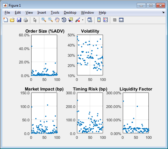
This figure demonstrates a snapshot view into the trading and liquidation
costs, volatility, and size of the stocks in the portfolio. You can modify this
scatter plot to include other variables from
TradeData.
See Also
krg | marketImpact | timingRisk | liquidityFactor