Sensitivity of Control System to Time Delays
This example shows how to examine the sensitivity of a closed-loop control system to time delays within the system.
Time delays are rarely known accurately, so it is often important to understand how sensitive a control system is to the delay value. Such sensitivity analysis is easily performed using LTI arrays and the InternalDelay property. For example, consider the notched PI control system developed in "PI Control Loop with Dead Time" from the example "Analyzing Control Systems with Delays." The following commands create an LTI model of that closed-loop system, a third-order plant with an input delay, a PI controller and a notch filter.
s = tf('s');
G = exp(-2.6*s)*(s+3)/(s^2+0.3*s+1);
C = 0.06 * (1 + 1/s);
T = feedback(ss(G*C),1);
notch = tf([1 0.2 1],[1 .8 1]);
C = 0.05 * (1 + 1/s);
Tnotch = feedback(ss(G*C*notch),1);
Examine the internal delay of the closed-loop system Tnotch.
Tnotch.InternalDelay
ans =
2.6000
The 2.6-second input delay of the plant G becomes an internal delay of 2.6 s in the closed-loop system. To examine the sensitivity of the responses of Tnotch to variations in this delay, create an array of copies of Tnotch. Then, vary the internal delay across the array.
Tsens = repsys(Tnotch,[1 1 5]);
tau = linspace(2,3,5);
for j = 1:5;
    Tsens(:,:,j).InternalDelay = tau(j);
end
The array Tsens contains five models with internal delays that range from 2.0 to 3.0.
Examine the step responses of these models.
stepplot(Tsens)
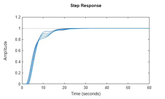
The plot shows that uncertainty on the delay value has a small effect on closed-loop characteristics.