Plotting System Responses

This example shows how to plot the time and frequency responses of SISO and MIMO linear systems.

Time Responses

Create a linear system. For this example, create a third-order transfer function.

sys = tf([8 18 32],[1 6 14 24])

sys =
 
     8 s^2 + 18 s + 32
  -----------------------
  s^3 + 6 s^2 + 14 s + 24
 
Continuous-time transfer function.

You can plot the step and impulse responses of this system using the step and impulse commands.

subplot(2,1,1)
step(sys)
subplot(2,1,2)
impulse(sys)

You can also simulate the response to an arbitrary signal, such as a sine wave, using the lsim command. The input signal appears in gray and the system response in blue.

figure
t = 0:0.01:4;
u = sin(10*t);
lsim(sys,u,t)   % u,t define the input signal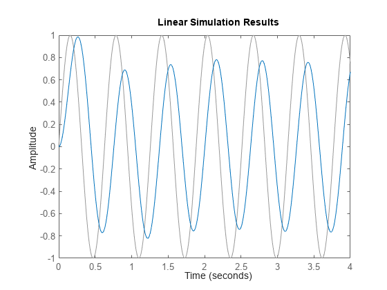

You can use the plotting commands with continuous or discrete tf, ss, or zpk models. For state-space models, you can also plot the unforced response from some given initial state. For example:

A = [-0.8 3.6 -2.1;-3 -1.2 4.8;3 -4.3 -1.1];
B = [0; -1.1; -0.2];
C = [1.2 0 0.6];
D = -0.6;
G = ss(A,B,C,D);
x0 = [-1;0;2];  % initial state
initial(G,x0)
grid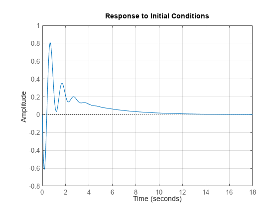

Frequency Responses

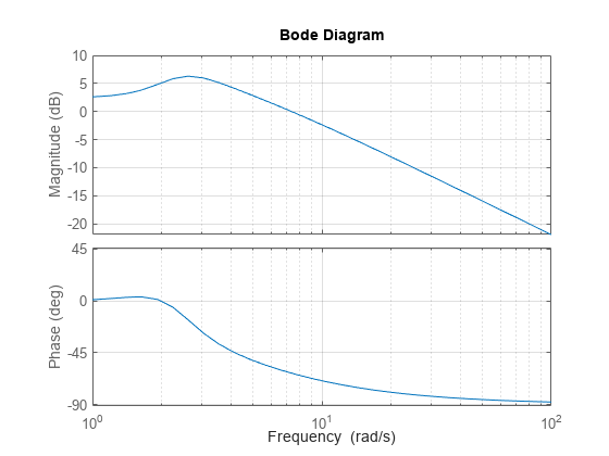
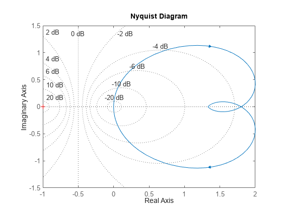
Frequency-domain analysis is key to understanding stability and performance properties of control systems. Bode plots, Nyquist plots, and Nichols charts are three standard ways to plot and analyze the frequency response of a linear system. You can create these plots using the bode, nichols, and nyquist commands.

Create a linear system.

sys = tf([8 18 32],[1 6 14 24])

sys =
 
     8 s^2 + 18 s + 32
  -----------------------
  s^3 + 6 s^2 + 14 s + 24
 
Continuous-time transfer function.

Create a Bode plot for this system.

bode(sys)
grid

Create a Nyquist plot for this system.

nyquist(sys)
grid

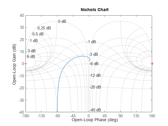
Create a Nichols chart for this system.

nichols(sys)
grid

Pole/Zero Maps and Root Locus

The poles and zeros of a system contain valuable information about its dynamics, stability, and limits of performance. For example, consider the feedback loop in the following SISO control loop.

Here:

$$G=\frac{-(2s+1)}{s^2+3s+2}$$

For the gain value k = 0.7, you can plot the closed-loop poles and zeros using pzmap.

s = tf('s');
G = -(2*s+1)/(s^2+3*s+2);
k = 0.7;
T = feedback(G*k,1);
pzmap(T)
grid
axis([-2 0 -1 1])

The closed-loop poles (marked by blue x's) lie in the left half-plane so the feedback loop is stable for this choice of gain k. You can read the damping ratio of the closed-loop poles from this chart (see labels on the radial lines). Here the damping ratio is about 0.7, suggesting a well-damped closed-loop response as confirmed by:

figure
step(T)

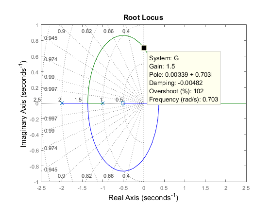
To further understand how the loop gain k affects closed-loop stability, you can plot the locus of the closed-loop poles as a function of k.

rlocus(G)
grid

Clicking where the locus intersects the y axis reveals that the closed-loop poles become unstable for k = 1.51. So the loop gain should remain smaller than 1.5 for closed-loop stability.

Response Characteristics

Right-clicking on response plots gives access to a variety of options and annotations. In particular, the Characteristics menu lets you display standard metrics such as rise time and settling time for step responses, or peak gain and stability margins for frequency response plots.

Using the example from the previous section, plot the closed-loop step response:

step(T)

Now, right-click on the plot to display the Peak Response and Settling Time Characteristics, and click on the blue dots to read the corresponding overshoot and settling time values:

Analyzing MIMO Systems

All commands mentioned so far fully support multi-input multi-output (MIMO) systems. In the MIMO case, these commands produce arrays of plots. For example, consider the following two-input, two-output system.

sys = rss(3,2,2);
sys.A = [-0.5 -0.3 -0.2 ; 0 -1.3  -1.7; 0.4 1.7 -1.3];

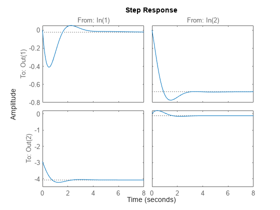
The step response is a 2-by-2 array of plots where each column shows the step response of a particular input channel.

step(sys)

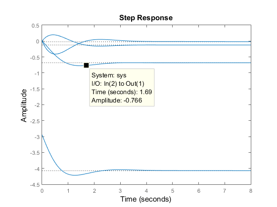
You can group all four responses on a single plot by right-clicking on the plot and selecting the I/O Grouping -> All submenu.

The following additional plots are useful for analyzing MIMO systems:

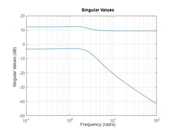
• Singular value plot (sigma), which shows the principal gains of the frequency response

• Pole/zero map for each I/O pair (iopzplot)

For example, plot the peak gain of sys as a function of frequency:

sigma(sys)
grid

Comparing Systems

You can plot multiple systems at once using any of the response plot commands. You can assign a specific color, marker, or line style to each system for easy comparison. Using the feedback example above, plot the closed-loop step response for three values of the loop gain k in three different colors:

k1 = 0.4;
T1 = feedback(G*k1,1);
k2 = 1;
T2 = feedback(G*k2,1);
step(T,'b',T1,'r',T2,'g')
legend('k = 0.7','k = 0.4','k = 1');

Modify Time or Frequency Axis Values

You can modify the time and frequency vectors for existing linear analysis plots.

For step and impulse plots, you can specify the time vector by right-clicking the plot area and selecting Specify time.

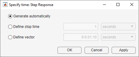
In the Specify time dialog box, you can define time values and units using one of the following methods.

• Generate automatically — Automatically generate the time vector based on the system dynamics. This option is not supported for sparse systems.

• Define stop time — Specify the stop time, which creates a time vector starting at time 0. The step size for the time vector is determined based on the system dynamics.

• Define vector — Specify the times to plot as a vector of monotonically increasing evenly spaced time values.

For bode, nyquist, nichols, and sigma plots, you can specify the frequency vector by right-clicking the plot area and selecting Specify frequency.

In the Specify frequency dialog box, you can define frequency values and units using one of the following methods.

• Generate automatically — Automatically generate the frequency vector based on the system dynamics. This method is not supported for sparse systems.

• Define range — Specify the frequency range. This method is not supported for sparse systems.

• Define vector — Specify the frequencies to plot as a vector.

If your system is an frd object, the plot interpolates the response between frequency values.

Changing the time and frequency units specifies the units for the input and does not change the units in the plot.