Model Array with Single Parameter Variation
This example shows how to create a one-dimensional array of transfer functions using the stack command. One parameter of the transfer function varies from model to model in the array. You can use such an array to investigate the effect of parameter variation on your model, such as for sensitivity analysis.
Create an array of transfer functions representing the following low-pass filter at three values of the roll-off frequency, a.
Create transfer function models representing the filter with roll-off frequency at a = 3, 5, and 7.
F1 = tf(3,[1 3]);
F2 = tf(5,[1 5]);
F3 = tf(7,[1 7]);
Use the stack command to build an array.
Farray = stack(1,F1,F2,F3);
The first argument to stack specifies the array dimension along which stack builds an array. The remaining arguments specify the models to arrange along that dimension. Thus, Farray is a 3-by-1 array of transfer functions.
Concatenating models with MATLAB® array concatenation commands, instead of with stack, creates multi-input, multi-output (MIMO) models rather than model arrays. For example:
G = [F1;F2;F3];
creates a one-input, three-output transfer function model, not a 3-by-1 array.
When working with a model array that represents parameter variations, You can associate the corresponding parameter value with each entry in the array. Set the SamplingGrid property to a data structure that contains the name of the parameter and the sampled parameter values corresponding with each model in the array. This assignment helps you keep track of which model corresponds to which parameter value.
Farray.SamplingGrid = struct('alpha',[3 5 7]);
Farray
Farray(:,:,1,1) [alpha=3] =
3
-----
s + 3
Farray(:,:,2,1) [alpha=5] =
5
-----
s + 5
Farray(:,:,3,1) [alpha=7] =
7
-----
s + 7
3x1 array of continuous-time transfer functions.
Model Properties
The parameter values in Farray.SamplingGrid are displayed along with the each transfer function in the array.
Plot the frequency response of the array to examine the effect of parameter variation on the filter behavior.
bodeplot(Farray)
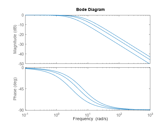
When you use analysis commands such as bodeplot on a model array, the resulting plot shows the response of each model in the array. Therefore, you can see the range of responses that results from the parameter variation.