Design Compensator Using Open-Loop Editor

Since R2025a

To design a compensator using a standalone open-loop editor created using openloopeditor, you interactively edit compensator poles, zeros, and gains. You can add dynamics and modify compensator parameters using the Compensator Editor or using the open-loop editor plot. In particular, you can:

• Adjust the compensator gain.

• Add real or complex-conjugate poles, including integrators.

• Add real or complex-conjugate zeros, including differentiators.

This topic describes how to design compensators using an open-loop editor. For more information on editing compensators in Control System Designer, see Edit Compensator Dynamics in Control System Designer.

Editor Views

In the open-loop editor, you can use the following views to design your compensator and switch between views for different perspectives on your design. To change the view, right click the plot area and select a view under View Type.

• Bode Editor — Using a Bode plot, you can adjust the open-loop bandwidth and design to gain and phase margin specifications.

• Nichols Editor — A Nichols plot combines gain and phase information into a single plot, which is useful when you are designing to gain and phase margin specifications. You can also use the Nichols plot grid lines to estimate the closed-loop response

• Root Locus Editor — View poles and zeros on a root locus plot. As the open-loop gain of the system varies, the root locus diagram shows the trajectories of the closed-loop poles of the closed-loop system.

You can also specify the view when you first open the open-loop editor using the ViewType property. For example, the following command opens the editor in the root locus view.

ole = openloopeditor(Plant=G,ViewType="rlocus");

Compensator Editor

To open the Compensator Editor dialog box, right click the open-loop editor plot area, and select Edit Compensator.

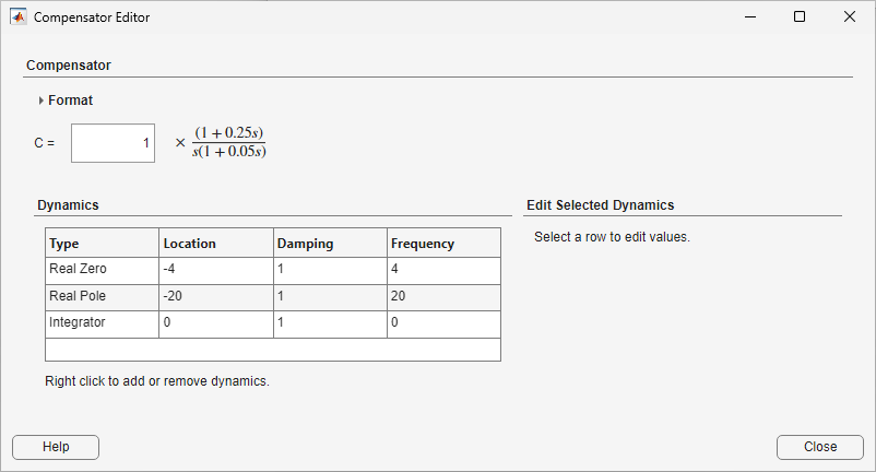
The Compensator Editor displays the current compensator transfer function. By default, the compensator transfer function displays in the time constant format. To change the format, under Format, in the drop-down, select one of these formats:

Format	Equations	Description
Time Constant	$$K\times \frac{\left(1+T_{z_1}s\right)\left(1+T_{z_2}s\right)}{\left(1+T_{p_1}s\right)\left(1+T_{p_2}s\right)}\cdots$$	K is the compensator DC gain. Tz1, Tz2, ..., are the zero time constants. Tp1, Tp2, ..., are the pole time constants.
Natural Frequency	$$K\times \frac{\left(1+s/{\omega }_{z_1}\right)\left(1+s/{\omega }_{z_2}\right)}{\left(1+s/{\omega }_{p_1}\right)\left(1+s/{\omega }_{p_2}\right)}\cdots$$	K is the compensator DC gain. ωz1, ωz2, … are the natural frequencies of the zeros. ωp1, ωp2, ..., are the natural frequencies of the poles.
ZPK	$$K\times \frac{\left(s+z_1\right)\left(s+z_2\right)}{\left(s+p_1\right)\left(s+p_2\right)}$$	K is the overall compensator gain. z1, z2, ... are the zero locations. p1, p2, ..., are the pole locations.

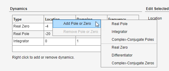
To add poles and zeros to your compensator, in the Compensator Editor, right-click the Dynamics table and, under Add Pole or Zero, select the type of pole or zero you want to add. The app adds a pole or zero of the selected type with default parameters.

To edit a pole or zero, in the Dynamics table, click on the pole/zero type you want to edit. Then, in the Edit Selected Dynamics section, in the text boxes, specify the pole and zero locations.

You can add the following poles and zeros to your compensator:

• Real pole/zero — Specify the pole/zero location on the real axis

• Complex conjugate poles/zeros — Specify complex conjugate pairs by:

  • Setting the real and imaginary parts directly.

  • Setting the natural frequency, ω_n, and damping ratio, ξ.

• Integrator — Add a pole at the origin to eliminate steady-state error for step inputs and DC inputs.

• Differentiator — Add a zero at the origin.

To delete poles and zeros, in the Dynamics table, right click on the pole or zero you want to delete and select Remove Pole or Zero.

Graphical Compensator Editing

You can also add and adjust poles and zeros directly from the open-loop editor plot. Use this method to roughly place poles and zeros in the correct area before fine-tuning their locations using the Compensator Editor.

In the plot, the editor displays the editable compensator poles and zeros as red X’s and O’s, respectively.

To add poles and zeros, use the toolbar that appears in the upper-right corner of the editor axes when you hover over the plot. To design a compensator, select these toolbar icons:

• — Add a real pole at the specified location.

• — Add a real zero at the specified location.

• — Add two complex conjugate poles at a specified location.

• — Add two complex conjugate zeros at a specified location.

• — Delete a pole or zero.

• — Display response data tips when you hover over or click the response.

When you do not have any toolbar icons selected, you can drag the response to adjust the compensator gain and you can drag the poles and zeros to adjust their locations. If you have the Compensator Editor open while dragging a pole or zero, you can view the new value in the Dynamics table.

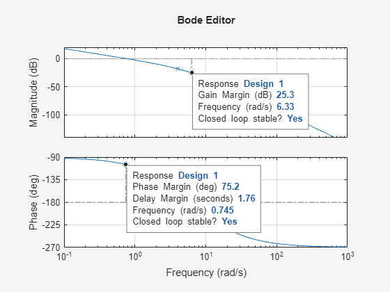
View Stability Margins

To view the gain and phase margins of the system in the open-loop editor:

1. Open either the Bode Editor or Nichols Editor view.

2. Right click the plot and select Characteristics > Minimum Stability Margins. The editor adds circular markers to the response indicating the locations of the gain and phase margins.

3. In the axes toolbar, click .

4. Hover over or click the margin locations in the plot. The resulting data tip shows the margin values and their corresponding frequencies. It also indicates whether the closed-loop system is stable.

View Closed-Loop Step Response

To view the closed-loop step response, you can extract the plant and compensator values from the OpenLoopEditor object and compute the closed-loop response using the feedback function.

Create the open-loop editor.

ole = openloopeditor(Plant=G);

After editing the compensator, compute the closed-loop response.

CL = feedback(ole.Plant*ole.Compensator,1);

Plot the closed-loop response.

stepplot(CL)

To automatically update a step plot when the compensator values change, you can specify the CompensatorChangingFcn and CompensatorChangedFcn properties of the OpenLoopEditor object. For an example, see Open-Loop Editor with Linked Step Plot.