Main Content

SparseModalTruncation

Sparse modal truncation model order reduction specification

Since R2023b

    Description

    The SparseModalTruncation object stores model order reduction specifications for the modal truncation of sparse linear time-invariant (LTI) models.

    For sparse modal truncation, unlike the ordinary modal truncation, you cannot compute all eigenvalues up front. The algorithm computes the N eigenvalues with smallest magnitude and then performs modal decomposition in this N-dimensional subspace. Hence, the modal decomposition is only approximate.

    G(s)D+k=1ncGk(s)

    By default, the algorithm computes the first 1000 modes, which can be very time consuming. But, you can limit the algorithm to compute a subset of modes based on the R.Options.Focus or R.Options.MaxOrder settings.

    Creation

    The reducespec function creates a modal truncation model order reduction object when you use this syntax.

    R = reducespec(sys,"modal")

    Here, sys is a sparse LTI model (sparss, mechss). The workflow uses this object to set up MOR tasks and store results. For the full model order reduction workflow, see Task-Based Model Order Reduction Workflow.

    Tip

    Computing all modes (poles) of sparse models is very time consuming. For best results, first set R.Options.Focus or R.Options.MaxOrder appropriately for your application to limit the number of modes to compute.

    Properties

    expand all

    This property is read-only.

    Average mode (pole) value in the subset of computed modal components Gk, returned as a vector of length nc-by-1, where nc is the number of computed modal components.

    This property is read-only.

    Damping ratio of average poles in the modal component Gk, returned as a vector of length nc-by-1, where nc is the number of computed modal components.

    This property is read-only.

    Natural frequency of average poles in the modal component Gk, returned as a vector of length nc-by-1, where nc is the number of computed modal components.

    This property is read-only.

    Computed model components Gk, returned as an nc-by-1 array of state-space models, where nc is the number of computed modal components.

    This property is read-only.

    Normalized DC contribution of modal components, returned as a vector of length nc-by-1, where nc is the number of computed modal components.

    These values are the DC gains of the computed modal components Gk(s) divided by the DC gain of the overall system. In some cases, the normalized DC contributions can exceed one if there are modal cancellations near DC (the overall DC gain is smaller than the sum of the DC contributions of each modal component).

    This property is read-only.

    Left-side matrix of block-diagonalizing transformation, returned as a matrix of size N-by-nc, where N is the number of states in the original model sys.

    The modal truncation algorithm transforms the state-space realization (A, B, C, D, E) of a model to block diagonal matrices (Am, Bm, Cm, Dm, Em) given by:

    • For explicit state-space models

      Am=TLTATR,Bm=TLTB,Cm=CTR,Dm=D,TLTTR=I

    • For descriptor state-space models

      Am=TLTATR,Bm=TLTB,Cm=CTR,Dm=D,Em=TLTETR

    Here, TL and TR are tall and skinny and project onto the invariant subspace associated with the computed modes.

    This property is read-only.

    Right-side matrix of block-diagonalizing transformation, returned as a matrix of size N-by-nc, where N is the number of states in the original model sys.

    The modal truncation algorithm transforms the state-space realization (A, B, C, D, E) of a model to block diagonal matrices (Am, Bm, Cm, Dm, Em) given by:

    • For explicit state-space models

      Am=TLTATR,Bm=TLTB,Cm=CTR,Dm=D,TLTTR=I

    • For descriptor state-space models

      Am=TLTATR,Bm=TLTB,Cm=CTR,Dm=D,Em=TLTETR

    Here, TL and TR are tall and skinny and project onto the invariant subspace associated with the computed modes.

    Options for modal truncation of sparse LTI models, specified as a SparseModalTruncationOptions object. Use dot notation to configure options for R. For example R.Options.Focus = [0,10000].

    For more information about available options, see SparseModalTruncationOptions.

    Object Functions

    processRun model order reduction algorithm
    view (modal)Plot mode information when using modal truncation method
    getrom (modal)Obtain reduced-order models when using modal truncation method

    Examples

    collapse all

    This example shows how to obtain a reduced-order model of a structural beam using the modal truncation method. For this example, consider a SISO sparse state-space model of a cantilever beam. This example uses the linearized model from the Linear Analysis of Cantilever Beam example.

    Load the beam model.

    load linBeam.mat
    size(sys)
    Sparse second-order model with 1 outputs, 1 inputs, and 3303 degrees of freedom.
    

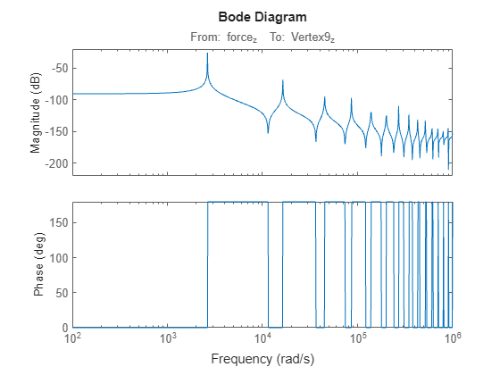
    Plot the Bode response.

    bode(sys,w)

    Create a model order reduction task.

    R = reducespec(sys,"modal");

    Set the Focus option to compute the eigenvalues only in the specified frequency range.

    R.Options.Focus = [0 5e5];

    Analyze the model and compute the derived information.

    R = process(R);
    size(R.Mode)
    ans = 1×2
    
        26     1


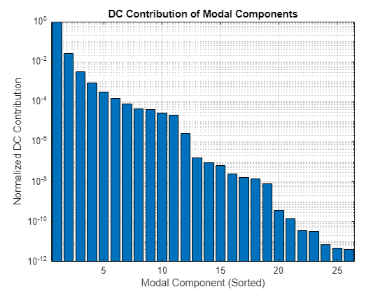
    The original model contains 26 modes. View the DC contribution of the modal components using the view function.

    view(R,"contrib")

    Discard the modes with smaller contributions. For this example, discard all modes with DC contribution smaller than 1e-6. This results in a reduced model with 12 modes.

    [rsys,info] = getrom(R,MinDC=1e-6);

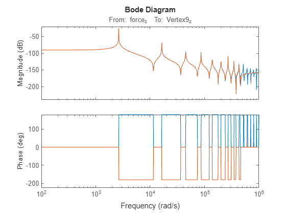
    Plot the bode responses.

    bode(sys,rsys,w)

    The reduced-order model provides a good approximation for the original sparse model.

    Algorithms

    Sparse modal truncation is applicable only to two types of symmetric semi-definite problems.

    • First-order problems with A = AT and E = ET semi-definite (positive or negative)

    • Second-order problems with K = KT, M = MT semi-definite (positive or negative), and Rayleigh damping C = αM + βK

    For both problems, the software uses the Krylov-Schur algorithm [1] to compute a subset of modes (see eigs).

    Once you decide which modes to keep and which modes to discard, the algorithm obtains the approximate modal decomposition G(s) = G1(s) + G2(s) + D, where G1(s) contains the desired modes. Then, based on the specified method, getrom returns the reduced-order model as follows.

    • "truncate"Gr(s) = G1(s) + D

    • "matchDC"Gr(s) = G1(s) + D + G2(0)

    References

    [1] Stewart, G. W. “A Krylov--Schur Algorithm for Large Eigenproblems.” SIAM Journal on Matrix Analysis and Applications 23, no. 3 (January 2002): 601–14. https://doi.org/10.1137/S0895479800371529.

    Version History

    Introduced in R2023b