SparseZeroPoleTruncation

Reduce sparse models using zero-pole truncation

Since R2025a

Description

The SparseZeroPoleTruncation object uses zero-pole truncation method to obtain low-order zero-pole-gain approximations of sparse state-space models. This method computes a subset of the zeros and poles of sparse models, typically in a specific low-frequency band [0 f_max]. It can yield better low-frequency approximations than modal truncation at the expense of more computation. This method also provides direct control over the roll-off slope past the frequency f_max.

Because this method calculates zeros for each input-output pair, it is most suitable for models with small input-output sizes. Additionally, this method is applicable only to models with a valid sparss representation.

Creation

The reducespec function creates a SparseZeroPoleTruncation model order reduction object when you use this syntax.

R = reducespec(sys,"zpk")

Here, sys is a sparse LTI model. The workflow uses this object to set up MOR tasks and store results. For the full workflow, see Task-Based Model Order Reduction Workflow.

Properties

Zero — Computed zeros

Read-only: [] (default) | cell array

This property is read-only.

Computed zeros in the specified frequency band, returned as an Ny-by-Nu cell array, where Ny is the number of outputs and Nu is the number of inputs in the model. Here, each entry of the cell array is a vector of real-valued or complex-valued zeros corresponding to that input-output channel.

Pole — Computed poles

Read-only: [] (default) | cell array

This property is read-only.

Computed poles in the specified frequency band, returned as an Ny-by-Nu cell array, where Ny is the number of outputs and Nu is the number of inputs in the model. Here, each entry of the cell array is a vector of real-valued or complex-valued poles of the model.

Gain — Computed gains

Read-only: [] (default) | array

This property is read-only.

Computed gains in the specified frequency band, returned as an Ny-by-Nu array, where Ny is the number of outputs and Nu is the number of inputs in the model. Here, each entry of the array is the real-valued or complex valued scalar gain corresponding to that input-output channel.

Options — Options for zero-pole truncation

SparseZeroPoleTruncationOptions object

Options for zero-pole truncation, specified as a SparseZeroPoleTruncationOptions object. Use dot notation to configure options for R. For example R.Options.Focus = [0 100].

For more information about available options, see SparseZeroPoleTruncationOptions.

Object Functions

view (zpk)	Plot computed poles and zeros when using zero-pole truncation method
getrom (zpk)	Obtain reduced-order models when using zero-pole truncation method

Examples

Reduce Sparse Beam Model Using Zero-Pole Truncation

This example shows how to obtain a reduced-order model of a structural beam using the zero-pole truncation method. For this example, consider a SISO sparse state-space model of a cantilever beam. This example uses the linearized model from the Linear Analysis of Cantilever Beam example.

Load the beam model.

load linBeam.mat
size(sys)

Sparse second-order model with 1 outputs, 1 inputs, and 3303 degrees of freedom.

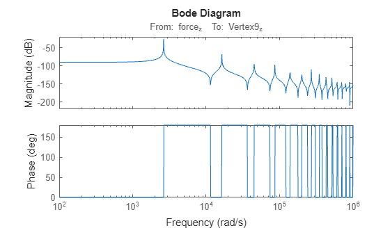
Analyze the frequency response of the model.

bodeplot(sys,w)

To perform sparse zero-pole truncation, first create a model order reduction task using reducespec with the "zpk" method.

R = reducespec(sys,"zpk");

For this task, set the frequency range of focus to compute modes up to 3e5 rad/s. Doing so prevents the algorithm from computing all the poles and zeros of the sparse model, which can take a long time in some cases.

R.Options.Focus = [0 3e5];
R.Options.Display = "off";

Run the model reduction algorithm. This computes the derived information, which are the poles, zeros, and gains of model, stored in the object R .

R = process(R);

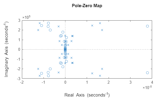
You can visualize the map of computed poles and zeros using the view function.

view(R)

Obtain the reduced zero-pole-gain approximation based on the specified frequency of focus.

rsys = getrom(R);
order(rsys)

ans = 
38

Compare the response of the original and reduced models.

figure;
opt = bodeoptions;
opt.PhaseWrapping = "on";
bodeplot(sys,rsys,"--",w,opt);

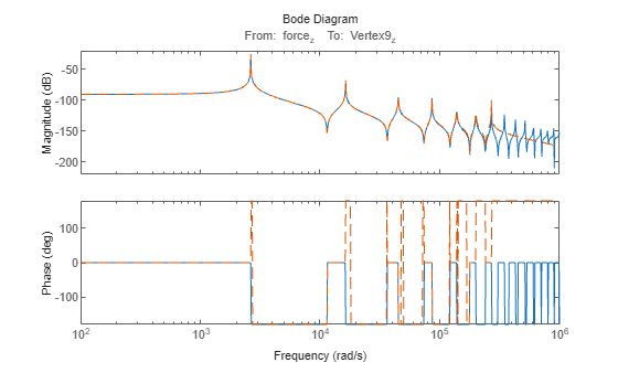
The reduced-order model provides a good approximation for the original sparse model in the specified range of interest.

Zero-Pole Truncation of Thermal Model

This example shows how to obtain a reduced model using zero-pole truncation of a sparse state-space model. This example uses a sparse model obtained from linearizing a thermal model of heat distribution in a circular cylindrical rod.

Load the model data.

load cylindricalRod.mat
sys = sparss(A,B,C,D,E);
w = logspace(-7,-1,20);
size(sys)

Sparse state-space model with 3 outputs, 1 inputs, and 7522 states.

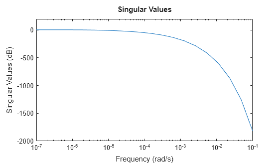
Analyze the frequency response of the model.

sigmaplot(sys,w)

Create a zero-pole truncation specification object for sys and specify the frequency band of focus. For this model, you can use a frequency range from 0 rad/s to 0.01 rad/s to obtain the low-order approximation.

R = reducespec(sys,"zpk");
R.Options.Focus = [0 1e-2];
R.Options.Display = "off";

Run the model reduction algorithm and obtain the reduced model.

R = process(R);
rsys = getrom(R);
sigmaplot(sys,rsys,w)

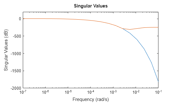
This thermal model has a very steep roll-off beyond 0.001 rad/s. By default, the reduced model obtained using getrom does not provide a good match for this roll-off. To mitigate this, you can use the RollOff argument of getrom and specify a minimum roll-off value beyond the frequency band of focus. Specify a roll-off slope value of -45, which corresponds to a rate of at least –900 db/decade.

rsys2 = getrom(R,RollOff=-45);
sigmaplot(sys,rsys2,w)

The reduced model now provides a much better approximation of the roll-off value.

Algorithms

This method uses the Krylov--Schur algorithm [1] for inverse power iterations to compute poles and zeros in the specified frequency band.

References

[1] Stewart, G. W. “A Krylov--Schur Algorithm for Large Eigenproblems.” SIAM Journal on Matrix Analysis and Applications 23, no. 3 (January 2002): 601–14. https://doi.org/10.1137/S0895479800371529.

Version History

Introduced in R2025a