Analyze Metal Conductors in Helical Dipole Antenna
This example shows how to design helical dipole antennas using different conductors and analyze their characteristics as functions of the conductor thickness and conductivity.
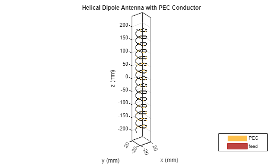
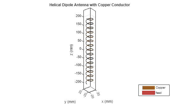
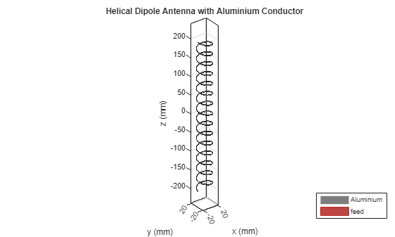
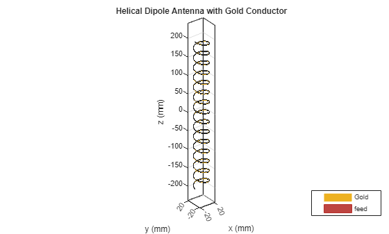
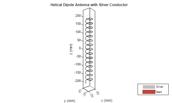
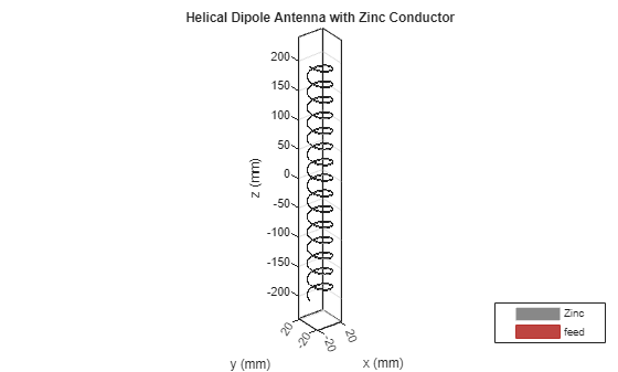
Create antennas with perfect electrical conductor (PEC), copper, aluminum, gold, silver, and zinc as the conducting materials. Create a row vector with the metal names and use the design function to create the antennas resonating at 1.8 GHz. Store the antennas in a row vector, in which the conductor of each antenna in the antennas vector corresponds to the material in the metals vector with the same index.
designFrequency = 1.8e9;
metals = ["PEC" "Copper" "Aluminium" "Gold" "Silver" "Zinc"];
antennas = repmat(dipoleHelix,size(metals));
for idx = 1:length(metals)
    helix = dipoleHelix(Conductor=metal(metals(idx)));
    antennas(idx) = design(helix,designFrequency);
    figure
    show(antennas(idx))
    title(sprintf("Helical Dipole Antenna with %s Conductor",metals(idx)))
end
Calculate Antenna Characteristics
Compute the impedance, directivity, gain, realized gain, return loss, and efficiency as functions of frequency for all the antennas. Store the values in a matrix in which each row corresponds to an antenna and each column corresponds to a frequency value.
freq = 1e9:50e6:3e9;
angles = 1:1:360;
z = zeros(length(antennas),length(freq));
loss = zeros(length(antennas),length(freq));
res = [1.4e9,1.8e9];
pat = zeros(length(antennas),length(res),length(angles));
eff = zeros(length(antennas),length(freq));
direct = zeros(length(antennas),length(freq));
gain = zeros(length(antennas),length(freq));
realizedgain = zeros(length(antennas),length(freq));
for idx = 1:length(antennas)
    ant = antennas(idx);
    z(idx,:) = impedance(ant,freq);
    [pat(idx,:,:),~,~] = pattern(ant,res,0,angles);
    direct(idx,:) = pattern(ant,freq,0,90,Type="directivity")';
    gain(idx,:) = pattern(ant,freq,0,90,Type="gain")';
    realizedgain(idx,:) = pattern(ant,freq,0,90,Type="realizedgain")';
    loss(idx,:) = returnLoss(ant,freq);
    eff(idx,:) = efficiency(ant,freq);
end
Vary Number of Turns
Vary the number of turns and determine whether the gain changes at azimuth and elevation angles of 0.
turns = 1:0.1:30;
pat2 = zeros(length(antennas),length(turns));
for idx = 1:length(metals)
    for jj = 1:length(turns)
        ant1 = dipoleHelix(Conductor=metal(metals(idx)));
        ant1.Turns = turns(jj);
        ant1 = design(ant1,designFrequency);
        pat2(idx,jj) = pattern(ant1,designFrequency,0,0);
    end
end
Vary Thickness
Vary the thickness of the conductor to compute impedance and efficiency. You cannot change the thickness of the PEC, because it has infinite conductivity and zero thickness, so omit PEC from the metals vector.
thicknesses = linspace(2e-7,1e-5,200);
z2 = zeros(length(antennas),length(thicknesses));
eff2 = zeros(length(antennas),length(thicknesses));
for idx = 2:length(metals)
    ant2 = dipoleHelix(Conductor=metal(metals(idx)));
    ant2 = design(ant2,designFrequency);
    for jj = 1:length(thicknesses)
        ant2.Conductor.Thickness = thicknesses(jj);
        z2(idx,jj) = impedance(ant2,designFrequency);
        eff2(idx,jj) = efficiency(ant2,designFrequency);
    end
end
Vary Conductivity
Vary the conductivity and calculate the return loss and gain. You cannot change the conductivity of the PEC, because it has infinite conductivity and zero thickness, so omit PEC from the metals vector.
conductivity = linspace(10e6,100e6,20);
loss2 = zeros(length(antennas),length(conductivity));
gain2 = zeros(length(antennas),length(conductivity));
for idx = 2:length(metals)
    for jj = 1:length(conductivity)
        ant3 = dipoleHelix(Conductor=metal(metals(idx)));
        ant3.Conductor.Conductivity = conductivity(jj);
        ant3 = design(ant3,designFrequency);
        loss2(idx,jj) = returnLoss(ant3,designFrequency);
        gain2(idx,jj) = pattern(ant3,designFrequency,0,90,Type="gain");
    end
end
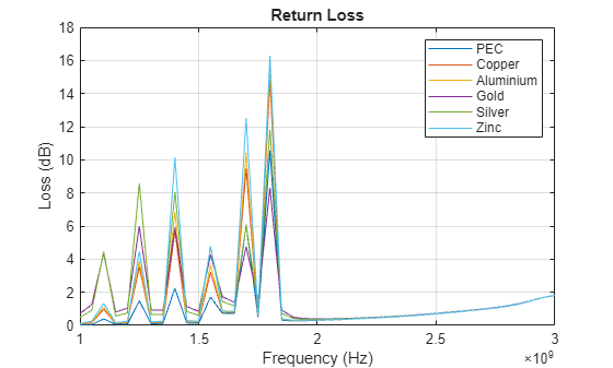
Plotting Impedance Against Frequency
Plot the impedance, directivity, gain, realized gain, return loss, and efficiency as functions of frequency. Because the frequency varies along the columns and the conductor varies along the rows, using the plot function results in 6 lines, one for each conductor.
figure
plot(freq,real(z))
grid on
title("Impedance")
xlabel("Frequency (Hz)")
ylabel("Resistance (Ohms)")
legend(metals)
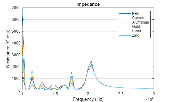
figure
plot(freq,imag(z))
grid on
title("Impedance")
xlabel("Frequency (Hz)")
ylabel("Reactance (Ohm)")
legend(metals)
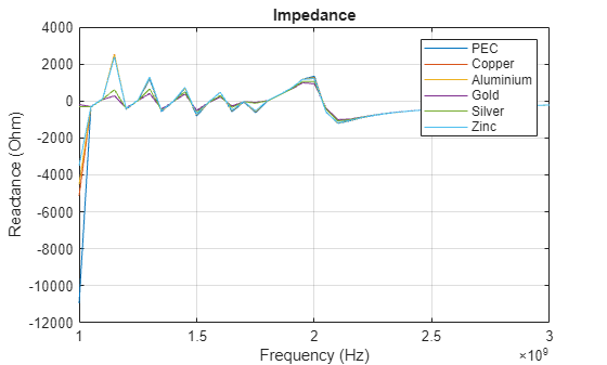
figure
plot(freq,loss)
grid on
title("Return Loss")
xlabel("Frequency (Hz)")
ylabel("Loss (dB)")
legend(metals)
To plot the gain, use the reshape function to convert the 6-by-1-by-360 pattern arrays to 6-by-360 pattern arrays.
for idx = 1:length(res)
    figure
    polarplot(angles*pi/180,reshape(pat(:,idx,:),[length(antennas),length(angles)]))
    title(sprintf("Gain (dBi) at %d Hz ",res(idx)));
    legend(metals)
end
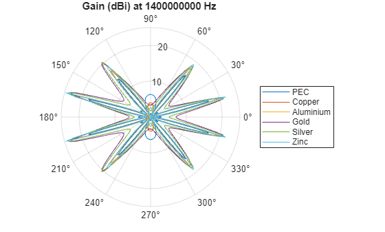
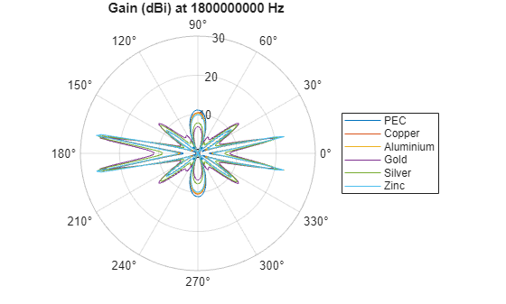
figure
plot(freq,eff)
grid on
title("Efficiency")
xlabel("Frequency (Hz)")
ylabel("Efficiency")
legend(metals)
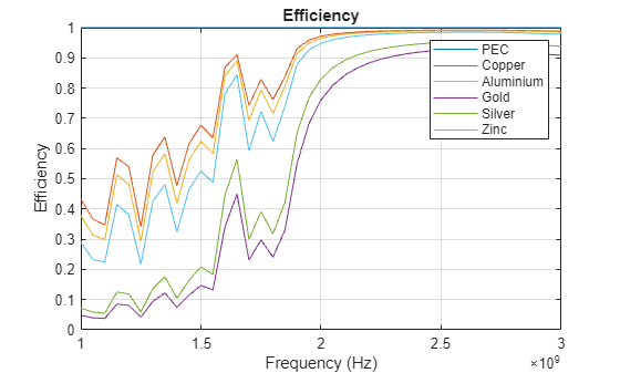
figure
plot(freq,direct)
grid on
title("Directivity")
xlabel("Frequency (Hz)")
ylabel("Directivity (dBi)")
legend(metals)
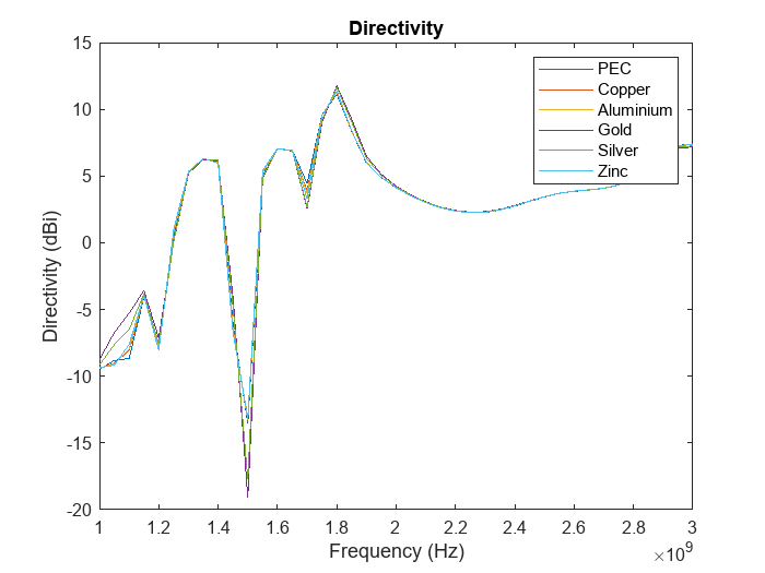
figure
plot(freq,gain)
grid on
title("Gain")
xlabel("Frequency (Hz)")
ylabel("Gain (dBi)")
legend(metals)
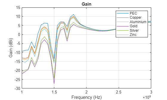
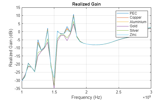
figure
plot(freq,realizedgain)
grid on
title("Realized Gain")
xlabel("Frequency (Hz)")
ylabel("Realized Gain (dBi)")
legend(metals)
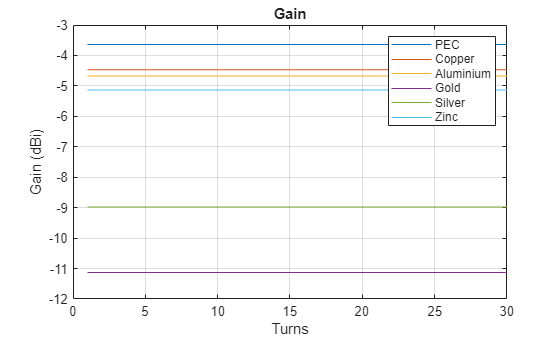
Plot Radiation Pattern Against Number of Turns
Plot the radiation pattern of each antenna as a function of the number of turns. The number of turns does not affect the gain of the antenna. The gain is constant for each conductor, regardless of the number of turns.
figure
plot(turns,pat2)
grid on
title("Gain")
xlabel("Turns")
ylabel("Gain (dBi)")
legend(metals)
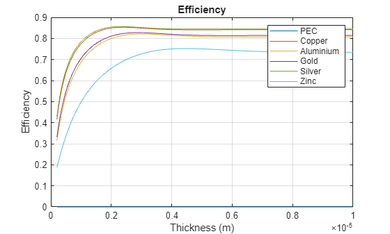
Plot Impedance and Efficiency Against Thickness
Plot the impedance and efficiency as functions of the thickness of the conductors.
figure
plot(thicknesses,real(z2))
grid on
title("Impedance")
xlabel("Thickness (m)")
ylabel("Resistance (Ohm)")
legend(metals)
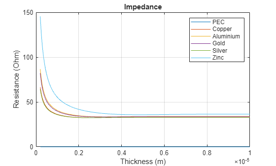
figure
plot(thicknesses,imag(z2))
grid on
title("Impedance")
xlabel("Thickness (m)")
ylabel("Reactance (Ohm)")
legend(metals)
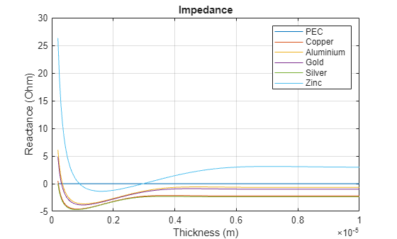
figure
plot(thicknesses,eff2)
grid on
title("Efficiency")
xlabel("Thickness (m)")
ylabel("Efficiency")
legend(metals)
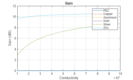
Plot Return Loss and Gain Against Conductivity
Plot the return loss and gain as functions of the conductivity of the conductors. Copper, aluminum, and zinc overlap on both plots. Gold and silver also overlap on both plots.
figure
plot(conductivity,loss2)
grid on
title("Return Loss")
xlabel("Conductivity (S/m)")
ylabel("Loss (dB)")
legend(metals)
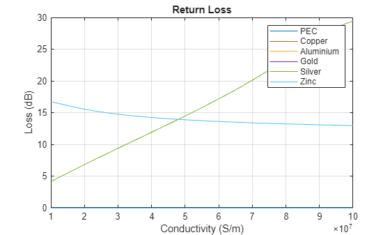
figure
plot(conductivity,gain2)
grid on
title("Gain")
xlabel("Conductivity")
ylabel("Gain (dBi)")
legend(metals)