Array Modeling and Analysis

This example shows how to create, visualize, and analyze an antenna array using the Antenna Toolbox™.

Create Antenna Array

Create a default rectangular antenna array using the rectangularArray object from the array catalog. By default, the array uses a dipole antenna as an element.

ra = rectangularArray

ra = 
  rectangularArray with properties:

           Element: [1×1 dipole]
              Size: [2 2]
        RowSpacing: 2
     ColumnSpacing: 2
           Lattice: 'Rectangular'
    AmplitudeTaper: 1
        PhaseShift: 0
              Tilt: 0
          TiltAxis: [1 0 0]

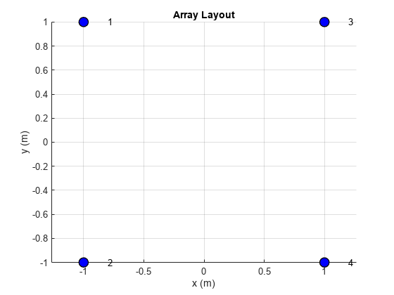
Visualize Array Layout

Use the layout function to plot the position of the array elements in the xy-plane. By default, the rectangular array is a 4-element dipole array in a 2-by-2 rectangular lattice.

layout(ra)

Visualize Array Geometry

Use the show function to view the structure of the rectangular antenna array.

figure
show(ra)
title("2-by-2 Rectangular Array of Dipoles");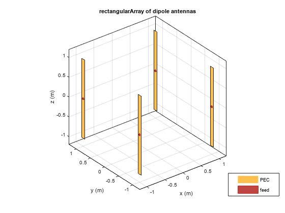

Plot Radiation Pattern of Array

Use the pattern function to plot the radiation pattern of the rectangular array. The radiation pattern is the spatial distribution of the radiated power of an array. The pattern displays the directivity or gain of the array. By default, the pattern function plots the directivity of the array.

figure
pattern(ra,70e6)

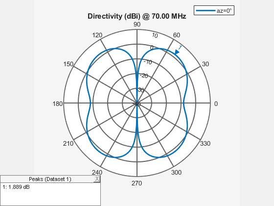
Plot Azimuth and Elevation Pattern of Array

Use patternAzimuth and patternElevation functions to plot the azimuth and elevation patterns of the rectangular array. These are the 2D radiation patterns of the array at a specified frequency.

figure
patternAzimuth(ra,70e6)

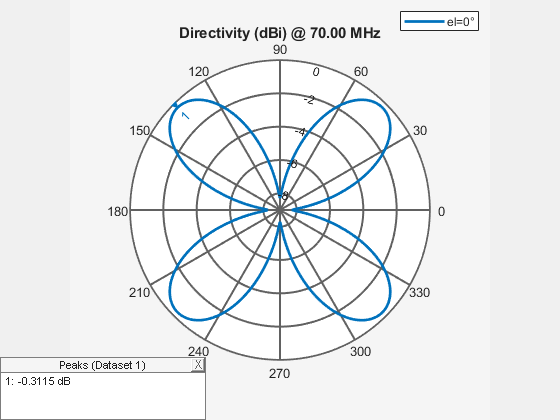
figure
patternElevation(ra,70e6)

Calculate Directivity of Array

Directivity is the ability of an array to radiate power in a particular direction. It can be defined as the ratio of the maximum radiation intensity in the desired direction to the average radiation intensity in all other directions. Use the pattern function to calculate the directivity of the rectangular array.

[Directivity] = pattern(ra,70e6,0,90)

Directivity = 
-39.5713

Calculate Electromagnetic Fields of Array

Use the EHfields function to calculate the electromagnetic fields of the rectangular array. This function returns the x, y, and z components of the electric and magnetic fields of the array. These components are measured at a specific frequency and at specified points in space.

[E,H] = EHfields(ra,70e6,[0;0;1])

E = 3×1 complex

   0.0000 + 0.0000i
   0.0003 + 0.0013i
  -1.3346 - 0.0736i

H = 3×1 complex
10-5 ×

   0.0186 - 0.2052i
   0.0000 + 0.0000i
   0.0000 + 0.0000i

Plot Array Radiation Pattern for Different Polarizations

Use the Polarization name-value argument in the pattern function to plot the different polarization patterns of the rectangular array. Polarization is the orientation of the electric field, or E-field, of an array. Polarization is classified as elliptical, linear, or circular. This example shows the left-hand circularly polarized (LHCP) radiation pattern of the rectangular array.

pattern(ra,70e6,Polarization="LHCP")

Calculate Beamwidth of Array

Use the beamwidth function to calculate the beamwidth of the rectangular array. The beamwidth of an array is the angular measure of the array pattern coverage. The beamwidth angle is measured in the plane that contains the direction of main lobe of the array.

[bw,angles] = beamwidth(ra,70e6,0,1:1:360)

bw = 4×1

   44.0000
   44.0000
   44.0000
   44.0000

angles = 4×2

    28    72
   108   152
   208   252
   288   332

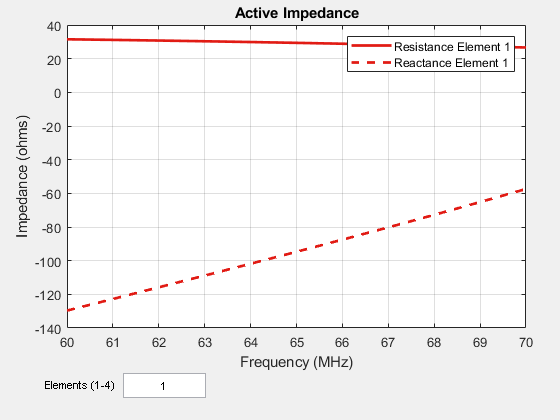
Calculate Scan Impedance of Array

Use the impedance function to calculate and plot the input impedance of rectangular array. Active impedance, or scan impedance, is the input impedance of each antenna element in an array, when all the elements are excited.

impedance(ra,60e6:1e6:70e6)

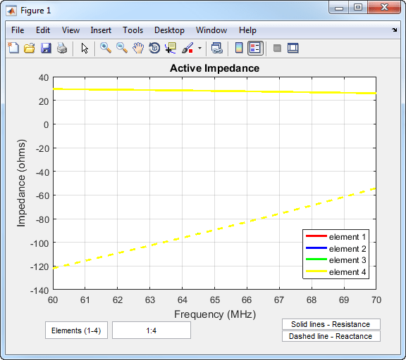
You can also view the impedance of all four elements by changing the number of elements on the plot from 1 to 1:4. See the following figure.

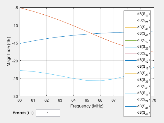
Calculate Reflection Coefficient of Array

Use the sparameters function to calculate the ${\mathit{S}}_{11}$ value of the rectangular array. ${\mathit{S}}_{11}$ value gives the reflection coefficient of the array.

S = sparameters(ra,60e6:1e6:70e6,72)

S = 
  sparameters with properties:

      Impedance: 72
       NumPorts: 4
     Parameters: [4×4×11 double]
    Frequencies: [11×1 double]

rfplot(S)

Calculate Return Loss of Array

Use the returnLoss function to calculate and plot the return loss of the rectangular array.

figure
returnLoss(ra,60e6:1e6:70e6,72)

You can also view the return loss of all four elements by changing the number of elements on the plot from 1 to 1:4. See the following figure.

Calculate Charge and Current Distribution of Array

Use the charge and current functions to calculate the charge and current distribution on the rectangular array surface.

figure
charge(ra,70e6)

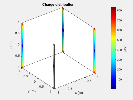
figure
current(ra,70e6)

Calculate Correlation Coefficient of Array

Use the correlation to calculate the correlation coefficient of the rectangular array. The correlation coefficient is the relationship between the incoming signals at the antenna ports in an array.

correlation(ra,60e6:1e6:70e6,1,2)

Change Size of Array and Visualize Layout

Use the Size property of the rectangular array to change it to a 16-element dipole array.

ra.Size = [4 4];
figure
show(ra)
title("4-by-4 Rectangular Array of Dipoles with Uniform Spacing");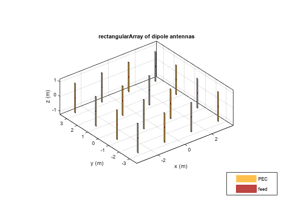

Change Array Elements Spacing to Nonuniform

Use the RowSpacing and ColumnSpacing properties of the rectangular array to change the spacing between the antenna elements.

ra.RowSpacing = [ 1.1 2 1.2];
ra.ColumnSpacing =[0.5 1.4 2]

ra = 
  rectangularArray with properties:

           Element: [1×1 dipole]
              Size: [4 4]
        RowSpacing: [1.1000 2 1.2000]
     ColumnSpacing: [0.5000 1.4000 2]
           Lattice: 'Rectangular'
    AmplitudeTaper: 1
        PhaseShift: 0
              Tilt: 0
          TiltAxis: [1 0 0]

figure
show(ra)
title("4-by-4 Rectangular Array of Dipoles with Nonuniform Spacing");

References

[1] Balanis, Constantine A. Antenna Theory: Analysis and Design. Fourth edition. Hoboken, New Jersey: Wiley, 2016.