Comparing Zonal Harmonic Gravity Model to Other Gravity Models

This example shows how to examine the zonal harmonic, spherical and 1984 World Geodetic System (WGS84) gravity models for latitudes from +/- 90 degrees at the surface of the Earth.

Determine Earth-Centered Earth-Fixed (ECEF) Position

Since ECEF coordinate system is geocentric, you can use spherical equations to determine the position from the latitude, longitude and geocentric radius.

Calculate the geocentric radii in meters at an array of latitudes from +/- 90 degrees using geocradius.

lat = -90:90;
r = geocradius( lat );
rlat = convang( lat, 'deg', 'rad');
z = r.*sin(rlat);

Because longitude has no effect for zonal harmonic gravity model, assume that the y position is zero.

x = r.*cos(rlat);
y = zeros(size(x));

Compute Zonal Harmonic Gravity for Earth

Use gravityzonal to calculate array of zonal harmonic gravity in ECEF coordinates for array of ECEF positions in meters per seconds squared.

[gx_zonal, gy_zonal, gz_zonal] = gravityzonal([x' y' z']);

Calculate WGS84 Gravity

Use gravitywgs84 to compute WGS84 gravity in down-axis and north-axis at the Earth's surface, an array of geodetic latitudes in degrees and 0 degrees longitude using the exact method with atmosphere, no centrifugal effects, and no precessing.

lat_gd = geoc2geod(lat, r);
long_gd = zeros(size(lat));
[gd_wgs84, gn_wgs84] = gravitywgs84( zeros(size(lat)), lat_gd, long_gd, 'Exact', [false true false 0] );

Determine Gravity for Spherical Earth

Compute the array of spherical gravity for the array of geocentric radii in meters per second squared using the Earth's gravitational parameter in meters cubed per second squared.

GM  = 3.986004415e14;
gd_sphere = -GM./(r.*r);

Comparison Plots for Different Gravity Models

To compare the gravity models, their outputs must be in the same coordinate system. You can transform zonal gravity from ECEF coordinates to NED coordinates by using the Direction Cosine Matrix from dcmecef2ned.

dcm_ef = dcmecef2ned( lat_gd, long_gd );
gxyz_zonal = reshape([gx_zonal gy_zonal gz_zonal]', [3 1 181]);
for m = length(lat):-1:1
    gned_zonal(m,:) = (dcm_ef(:,:,m)*gxyz_zonal(:,:,m))';
end

figure(1)
plot(lat_gd, gned_zonal(:,3), lat, -gd_sphere, '--', lat_gd, gd_wgs84, '-.')
legend('Zonal Harmonic', 'Spherical', 'WGS84','Location','North')
xlabel('Geodetic Latitude (degrees)')
ylabel('Down gravity (m/s^2)')
grid

Figure 1: Gravity in the Down-axis in meters per second squared

figure(2)
plot( lat_gd, gned_zonal(:,1), lat_gd, gn_wgs84, 'r-.' )
hold on
plot([lat(1) lat(end)], [0 0], 'g--' )
legend('Zonal Harmonic', 'WGS84', 'Spherical','Location','Best')
xlabel('Geodetic Latitude (degrees)')
ylabel('North gravity (m/s^2)')
grid
hold off

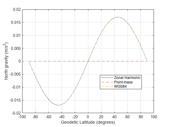
Figure 2: Gravity in the North-axis in meters per second squared

Calculate total gravity for WGS84 and from zonal gravity vector in meters per second squared.

gtotal_wgs84 = gravitywgs84( zeros(size(lat)), lat_gd, zeros(size(lat)), 'Exact', [false true false 0] );
gtotal_zonal = sqrt(sum([gx_zonal.^2 gy_zonal.^2 gz_zonal.^2],2));

figure(3)
plot( lat, gtotal_zonal, lat_gd, gtotal_wgs84, '-.' )
legend('Zonal Harmonic', 'WGS84','Location','North')
xlabel('Geodetic Latitude (degrees)')
ylabel('Total gravity (m/s^2)')
grid

Figure 3: Total gravity in meters per second squared

Compare Gravity Models with Centrifugal Effects

Now, you have seen the gravity comparisons of a non-rotating Earth. Examine the centrifugal effects from the Earth's rotation on the gravity models.

Compute Gravity Centrifugal Effects for Earth

Use gravitycentrifugal to calculate array of centrifugal effects in ECEF coordinates for array of ECEF positions in meters per seconds squared.

[gx_cent, gy_cent, gz_cent] = gravitycentrifugal([x' y' z']);

Add centrifugal effects to zonal harmonic gravity.

gx_cent_zonal = gx_zonal + gx_cent;
gy_cent_zonal = gy_zonal + gy_cent;
gz_cent_zonal = gz_zonal + gz_cent;

Calculate WGS84 Gravity with Centrifugal Effects

Use gravitywgs84 to compute WGS84 gravity in down-axis and north-axis at the Earth's surface, an array of geodetic latitudes in degrees and 0 degrees longitude using the exact method with atmosphere, centrifugal effects, and no precessing.

[gd_cent_wgs84, gn_cent_wgs84] = gravitywgs84( zeros(size(lat)), lat_gd, long_gd, 'Exact', [false false false 0] );

Calculate total gravity with centrifugal effects for WGS84 and from zonal gravity vector in meters per second squared.

gtotal_cent_wgs84 = gravitywgs84( zeros(size(lat)), lat_gd, zeros(size(lat)), 'Exact', [false false false 0] );
gtotal_cent_zonal = sqrt(sum([gx_cent_zonal.^2 gy_cent_zonal.^2 gz_cent_zonal.^2],2));

Comparison Plots for Different Gravity Models with Centrifugal Effects

To compare the gravity models, their outputs must be in the same coordinate system. You can transform zonal gravity from ECEF coordinates to NED coordinates by using the Direction Cosine Matrix from dcmecef2ned. In figure 5, you can see there is some difference between zonal harmonic gravity with centrifugal effects and WGS84 gravity with centrifugal effects. The majority of difference is due to differences between the zonal harmonic gravity and WGS84 gravity calculations.

gxyz_cent_zonal = reshape([gx_cent_zonal gy_cent_zonal gz_cent_zonal]', [3 1 181]);
for m = length(lat):-1:1
    gned_cent_zonal(m,:) = (dcm_ef(:,:,m)*gxyz_cent_zonal(:,:,m))';
end

figure(4)
plot(lat_gd, gned_cent_zonal(:,3), lat_gd, gd_cent_wgs84, '-.')
legend('Zonal Harmonic', 'WGS84','Location','North')
xlabel('Geodetic Latitude (degrees)')
ylabel('Down gravity (m/s^2)')
grid

Figure 4: Gravity with centrifugal effects in the Down-axis in meters per second squared

figure(5)
plot( lat_gd, gned_cent_zonal(:,1), lat_gd, gn_cent_wgs84, '--', lat_gd, (gned_zonal(:,1)-gn_wgs84'), '-.' )
axis([-100 100 -0.0002 0.0002])
legend('Zonal Harmonic', 'WGS84', 'Error Between Models w/o Centrifugal Effects', 'Location','Best')
xlabel('Geodetic Latitude (degrees)')
ylabel('North gravity (m/s^2)')
grid

Figure 5: Gravity in the North-axis in meters per second squared

figure(6)
plot( lat, gtotal_cent_zonal, lat_gd, gtotal_cent_wgs84, '-.' )
legend('Zonal Harmonic', 'WGS84','Location','North')
xlabel('Geodetic Latitude (degrees)')
ylabel('Total gravity (m/s^2)')
grid

Figure 6: Total gravity with centrifugal effects in meters per second squared

×

Open Example

You have a modified version of this example. Do you want to open this example with your edits?

No, overwrite the modified version Yes