Modeling and Simulation of an Autonomous Underwater Vehicle

This example uses:

This example shows how to simulate the dynamics and control of an autonomous submarine using Simulink® and the Aerospace Blockset™. Given a reference heading trajectory, this example designs a control law enabling the autonomous submarine to obey the reference parameters.

Examples of the use of autonomous underwater vehicles include deep-sea geological surveying, exploration, and search and rescue. Autonomizing these vehicles saves the weight of a human crew, reducing the overall mission cost and increasing the scope of mission objectives (for example, enabling large sample returns or enabling more fuel to be stored on board, which can lead to a longer mission duration).

For the purposes of this example, all motion is performed via propulsion, without the use of control surfaces.

Assuming values for the timeseries heading reference and the vehicle current and velocity, the controller calculates appropriate thrust commands to pass to the plant for actuation. These forces and moments act on the vehicle to drive its current heading to the reference heading.

Modeling Assumptions

Assume that the submarine is torpedo-shaped. For underwater propulsion, the vehicle uses thrusters of two different sizes, T200 and T100). In total, the vehicle uses five thrusters arranged as follows:

Two T200 thrusters provide forward thrust rated at 66N each
Two T100 thrusters provide pitch moments rated at 33N each
Two T100 thrusters provide yaw moments rated at 33N each

Assume that all thrusters in a group operate identically. For example, the two T200 thrusters intended to provide surge always provide identical amounts of thrust at any given instant of time. This means that they cannot be individually commanded to produce different thrusts. The T100 thrusters produce moments by pushing in opposite directions, always with the same thrust.

Assume that the submarine is always fully submerged in the water. This means that the vehicle does not resurface and therefore no component of the vehicle interacts with air above the water.

Open the Model

open_system("asbAUV");

The top level diagram closely resembles the high-level workflow presented in the introduction.

The model has these simulation options:

System Without Noise/System With Noise - Enable or suppress the presence of noise in the sensor measurements.
Off/Low/High - Specify quality of visualization.

"Off" runs without visualization
"Low" runs with a live MATLAB
"High" renders a 3D scene using Unreal Engine

The model always runs in high fidelity mode for modeling of the propulsion forces.

Control Strategy

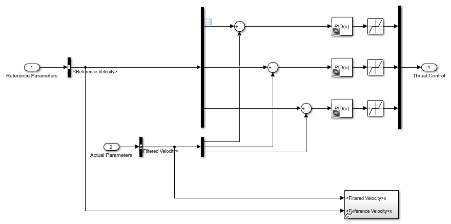
The "GNC" (Guidance, Navigation, and Control) subsystem contains the sensor model and controllers that allow the AUV to follow a given reference heading. A Signal Editor block generates a timeseries reference heading for the vehicle to follow. This reference heading signal is input into the PID attitude controller which outputs commanded moments on the vehicle. The reference roll angle is held at a constant, and the reference pitch angle is determined by the difference between the desired dive depth and vehicle depth.

open_system("asbAUV/GNC/Attitude Controller")

A PID speed controller acts on the error between the vehicle's forward speed and a constant desired cruise speed to output desired thrust.

open_system("asbAUV/GNC/Speed Controller")

The resulting thrust and moment commands are then passed to the plant and actuator models to calculate the actuator forces and moments on the vehicle.

Vehicle and Environment Modeling

The "Plant" system calculates both environmental and propulsive forces, including hydrostatic, hydrodynamic, and gravitational forces and moments.

Hydrostatic force is the buoyant force and hydrodynamic moment multiplied by the moment arm from the center of buoyancy to the center of mass. Because the vehicle is assumed to always be submerged, this force does not consider the air above the waterline.

open_system("asbAUV/AUV_Plant/Environmental Forces and Moments /Hydrostatic")

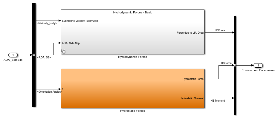
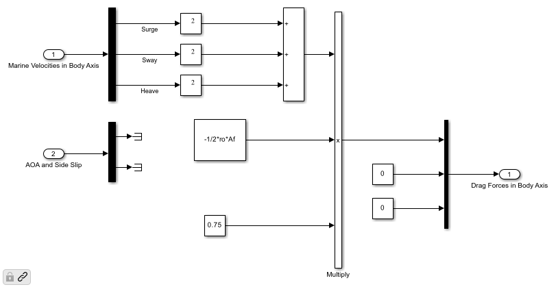
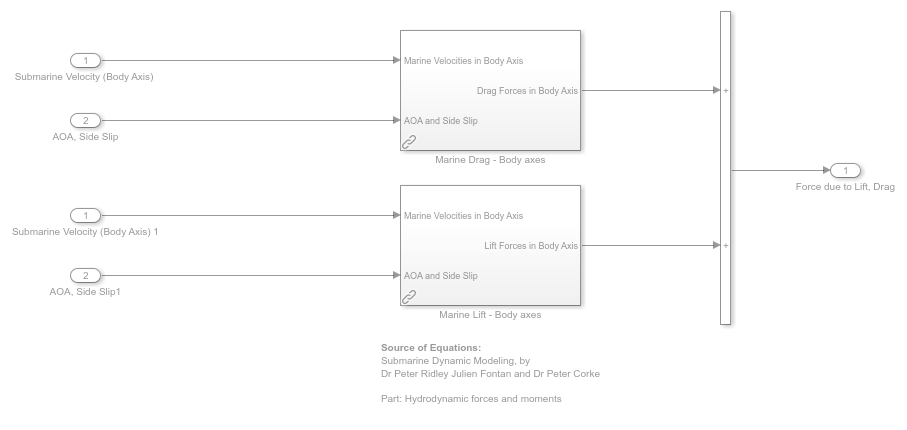
The example calculates hydrodynamic forces and moments using lookup tables for six coefficients, which depend on the angle of attack and sideslip. To dimensionalize the nondimensional coefficients, the examples passes the coefficients and the dynamic pressure and vehicle size to an Aerodynamic Forces and Moments block.

For small rotation rates, these six coefficients provide accurate forces and moments. However, viscous damping due to rotation is significant in water. For this reason, theis example also provides a linear damping model.

open_system("asbAUV/AUV_Plant/Environmental Forces and Moments /Hydrodynamic")

The "Actuators" subsystem calculates propulsive forces and moments. This block takes the force and moment on the vehicle and converts it to individual thrust commands for each thruster. This model has two levels of fidelity.

open_system("asbAUV/AUV_Plant/Actuators/Actuators (high fidelity)")

The level of simulation fidelity determines the subsystem that is activated.

High Fidelity Simulation: Include experimentally determined transfer functions for the T100 and T200 thrusters.
Low Fidelity Simulation: Ignores transient effects like spool-up time, which increases the performance of the thrusters but reduces accuracy.

To solve for the dynamics, the model sums together the computed hydrodynamic, hydrostatic, gravitational, and previously computed propulsion forces and moments and passes the total to the 6DOF block. This block computes the states of the vehicle at the next time step. These states include position and velocity in body and flat-earth frame, Euler angles, direction cosines matrix, and angular velocity.

open_system("asbAUV/AUV_Plant")

The model then groups these states into a bus signal called "state". This state captures all important information about the vehicle at each time step. The model feeds "state" to both the visualization and GNC subsystems.

Sensor Data and State Estimation

The "State Estimator" subsystem mimics a sensor measurement. It demonstrates the use of filters to remove noise by introducing noise into the vehicle current motion parameters.

open_system("asbAUV/GNC/State Estimator/State Estimator (with noise)");

When noise is off, the "State Estimator (without noise)" block works as a passthrough, giving the controller perfect full state information. When noise is on, the "State Estimator" subsystem switches to a different variant. In this subsystem, the IMU block is used to model a gyroscope and accelerometer with noisy measurements.

open_system("asbAUV/GNC/State Estimator/State Estimator (with noise)/IMU");

The IMU Measurements signal is separated back into measured acceleration and measured angular rates. Each quantity has three components (x, y, and z) which are passed through a lowpass filter to obtain a best estimate of the relevant quantity. These components are integrated over time to obtain filtered quantities of the vehicle's position, velocity, orientation angles, and angular rates in the body frame.

open_system("asbAUV/GNC/State Estimator/State Estimator (with noise)/Internal filter")

These filtered quantities are then passed to the controllers to compute desired forces and moments.

Why Use the Aerospace Blockset?

Hand-modeling six coupled equations of motion in Simulink is prone to errors. To reduce the chance of modeling errors arising from this, use the 6DOF block from the Aerospace Blockset. The 6DOF block computes the following position data, given the total force and moment acting on a body:

Vehicle velocity in the flat Earth frame
Vehicle position in the flat Earth frame
Euler rotation angles
The direction cosine matrix relating the body frame to the flat Earth frame
Vehicle velocity in the body-fixed frame
Angular velocity of the vehicle in the body-fixed frame

The above outputs are in different reference frames, which may not be ideal for some applications. To ensure that quantities remain in desired reference frames, use the rotation and coordinate transformation blocks.

For convenience, convert Euler rotation angles to direction cosine matrix elements and vice versa. To achieve this, use the Direction Cosine Matrix to Rotation Angles and Rotation Angles to Direction Cosine Matrix blocks.

The Three-axis Inertial Measurement Unit block is useful in the state estimation part of the problem. Given the vehicle's actual acceleration, angular rates, angular accelerations, center of gravity location, and the acceleration due to gravity, the block mimics an IMU and outputs measured values of the vehicle's acceleration and angular rates.

The Aerospace Blockset also lets you simulate a 6DOF system in which the vehicle's mass is variable. This capability lets you model fuel consumption as the simulation runs, resulting in a more accurate model. Other available functionalities include actuators, aerodynamics simulations, instrument modeling, center of gravity estimation, etc.

Simulation - Heading Reference

asbHeadingScenario.mat provides an example heading trajectory. This trajectory consists of a smooth right turn and then left turn while holding a constant depth of about 2m.

Click the 'Run' button or press Ctrl+T. After compilation, the model runs and a figure window or Unreal Engine window opens showing the vehicle's live position and rotation. The gauges show the speed, depth, and attitude of the vehicle.

Alternate Control Strategies

The control problem illustrated by this example can be further extended to be an optimal control problem. In other words, as opposed to merely controlling the position and velocity of the vehicle, the controller must now control the position and velocity while simultaneously satisfying another set of constraints. For example, keeping the vehicle on a known path while minimizing fuel consumption. In view of this, two alternate control strategies can be used, model predictive control and linear quadratic regulator.

Model Predictive Control

Using a model predictive controller, a finite time-horizon is computed. For each time step leading up to the horizon, the optimal control input for the current time step is computed (via linearizing the model at the current time step), actuated, and then reoptimized to the new time-horizon until the end of the simulation. The main advantage of this control strategy over PID is that the optimization of the control input required for the current time step takes into consideration the future time steps. Furthermore, this enables the controller to anticipate future events and effect appropriate control measures. This control strategy is particularly useful if the vehicle is to automatically detect and avoid obstacles.

Linear Quadratic Regulator

A linear quadratic regulator (LQR) is also a good candidate for a control strategy in such an optimal control problem. Using an LQR involves computing the optimal control inputs that minimize a specified quadratic cost function. In this specific problem, the cost function can be the amount of fuel used that must be minimized. The difference between this and model predictive control is that an LQR optimizes over the entire time horizon of the simulation, while an MPC uses a receding horizon. An advantage of LQR over MPC lies in the lower amount of computational power required.