Collision Avoidance Maneuver for Upcoming Conjunction

This example shows how to identify and avoid an upcoming conjunction. The example use two-line elements (TLEs) to identify the conjunction. It then shows how to use a satellite maneuver with Aerospace Blockset™ to avoid the conjunction. The example uses the Orbit Propagator block to calculate the trajectory after the maneuver.

Disclaimer - Do not use publicly available TLEs for operational conjunction assessment prediction and avoidance. This example is provided for informational purposes only. Satellite operators should contact the 18th Space Defense Squadron for data and analysis to support operational satellites.

Introduction

Due to the large constellations launched in the last few years, satellite conjunctions that require avoidance maneuvers are a common problem in Low Earth Orbit (LEO). In return, satellite operators must respond to conjunction messages received from 18th Space Control Squadron and provide updated ephemerides. NASA addresses this issue in their Best Practices Handbook [1] and the Space Control Squadron in their Spaceflight Safety Handbook for Satellite Operators [2]. Avoidance maneuvers are very small maneuvers, typically along the track of the orbit, to maximize distance from the potential conjunction, as described in [3].

Notes:

• This example uses a Starlink satellite.

• All computations in this example are performed in the inertial frame.

Tools used:

• To find upcoming conjunctions between a pair of objects using their Two-Line Elements, or TLEs, we first use findConjunctions() function using the satellite() and states() functions from the Aerospace Toolbox.

• To find upcoming conjunctions, we use the SOCRATES online tool from the Celestrak website. The probability of the conjunction is computed both before and after the planned avoidance maneuver.

• To compute a maneuver from the desired radial offset and determine the expected tangential miss distance, we use an approximate analytic solution [3]. This is equivalent to the first portion of a Hohmann transfer to a slightly higher orbit, which provides both radial and tangential distance from the original conjunction location.

• To simulate the orbit of the active satellite, we use the Orbit Propagator block. The orbit of the debris is propagated using its TLE. The TLEs must be accurate within about a kilometer for the time frame of interest, which is up to seven days. The reference orbit and the perturbed orbit is used to plot the relative distance between the maneuvering satellite and the conjunction point.

Identify Upcoming Conjunctions

We use an example with a Starlink satellite and CZ-2D DEB debris. The TLE pair for the satellite and debris is saved into a text file.

mission.tleFile = 'Conjunction_Starlink1079_CZ2DDeb.txt';
type Conjunction_Starlink1079_CZ2DDeb.txt

STARLINK-1079
1 44937U 20001Z   22272.52136386 -.00000745  00000+0 -31120-4 0  9997
2 44937  53.0548 210.2777 0001443  83.0631 277.0522 15.06393387150649
CZ-2D DEB
1 43406U 12073D   22272.74034628  .00008296  00000+0  83006-3 0  9993
2 43406  97.9471 196.5364 0090895 225.9886 133.3815 14.88613293478469

Load the TLE into a Scenario

Load the elements into a scenario object and print the orbital elements for inspection. Both satellites are set up with the SGP4 propagator. We save the start time of the scenario for later use.

mission.sc  = satelliteScenario;
mission.sat = satellite(mission.sc,mission.tleFile); % two satellites
mission.sat(2).MarkerColor = [1 0.059 1];
mission.sat(2).Orbit.LineColor = [1 0.059 1];
mission.startTime = mission.sc.StartTime;
mission.elements(1) = orbitalElements(mission.sat(1));
mission.elements(2) = orbitalElements(mission.sat(2));

The satellites orbital elements, from the TLEs, are displayed below. Note satellite 1, the StarLink satellite, has a negative BStar, which is a form of the ballistic coefficient. Negative values can happen due to the averaging process used to generate TLEs. In this case, it means that drag has a very small impact on the location of this satellite over our period of interest, up to seven days from epoch. The debris object has an order of magnitude larger (positive) BStar. The debris object also has an order of magnitude higher eccentricity.

mission.elements(1)

ans = struct with fields:
                       MeanMotion: 0.0628
                     Eccentricity: 1.4430e-04
                      Inclination: 53.0548
    RightAscensionOfAscendingNode: 210.2777
              ArgumentOfPeriapsis: 83.0631
                      MeanAnomaly: 277.0522
                           Period: 5.7356e+03
                            Epoch: 29-Sep-2022 12:30:45
                            BStar: -3.1120e-05

mission.elements(2)

ans = struct with fields:
                       MeanMotion: 0.0620
                     Eccentricity: 0.0091
                      Inclination: 97.9471
    RightAscensionOfAscendingNode: 196.5364
              ArgumentOfPeriapsis: 225.9886
                      MeanAnomaly: 133.3815
                           Period: 5.8041e+03
                            Epoch: 29-Sep-2022 17:46:05
                            BStar: 8.3006e-04

Find the Conjunctions

Next, find the conjunctions using the findConjunctions function. This may take a minute or two depending on the number of close intersections of the orbits within the screening period. The two-step process first uses a coarse propagation with the screening distance to find conjunction windows. A search then finds the closest distance within each window.

nDaysDouble = 7;
nDays = days(nDaysDouble);
dScreen = 200000;
dMin = 1000;
[conj.tCA,conj.missDistance,conj.relVelocity] = findConjunctions(mission.sc,...
  mission.sat(1),mission.sat(2),nDays,dScreen,dMin);
disp(table(conj.tCA, conj.missDistance, conj.relVelocity, days(conj.tCA-mission.startTime), ...
  VariableNames=["Conjunction time", "Dist at closest approach (m)", "Velocity difference (m/s)", "Time from epoch (days)"]))

      Conjunction time      Dist at closest approach (m)    Velocity difference (m/s)    Time from epoch (days)
    ____________________    ____________________________    _________________________    ______________________

    03-Oct-2022 08:06:49               17.174                        5861.3                      3.8167        

We need the states at the time of closest approach.

[conj.X_icrf,conj.V_icrf] = states(mission.sat,conj.tCA(1),CoordinateFrame='inertial'); % m/s

Visualize at Time of Closest Approach

View the satellite, STARLINK-1079, and debris, CZ-2D DEB, orbits in the scenario viewer. This zoomed-in view at the time of closest approach shows that the satellite and debris have a probable conjunction.

viewerMission= satelliteScenarioViewer(mission.sc,"CurrentTime",conj.tCA);
camheight(viewerMission, 9.0e+05);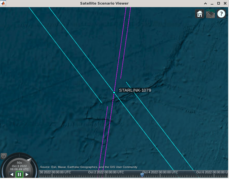

Conjunction Probability

As described in the NASA handbook, the conjunction probability can be computed using integration with quad2D(). This requires knowledge or an estimate of the covariance of both objects and their hard-body radii. If the predicted miss distance is within the combined hard-body radii of the satellites, the probability is 1. Otherwise, the combined covariances are integrated over this hard-body sphere. This integration is shown in the plot generated below with the drawConjunction function. The miss distance of the secondary object is on the x-axis and the primary object's motion is along the y-axis. The axes of the encounter frame are computed from the differences in position and velocity and their cross-product, $\Delta \overrightarrow{\mathit{r}}=\overrightarrow{{\mathit{r}}_1}-\overrightarrow{{\mathit{r}}_2}$, $\Delta \overrightarrow{\mathit{v}}\equiv \overrightarrow{\mathit{y}}=$$\overrightarrow{{\mathit{v}}_1}$-$\overrightarrow{{\mathit{v}}_2}$, $\overrightarrow{\mathit{h}}\equiv \overrightarrow{\mathit{z}}=\Delta \overrightarrow{\mathit{r}}\times \Delta \overrightarrow{\mathit{v}}$, $\overrightarrow{\mathit{x}}=\overrightarrow{\mathit{y}}\times \overrightarrow{\mathit{z}}$. The covariance defines the one-sigma ellipse, shown with the red dashed line.

cov2x2 = [1 -0.6; -0.6 2]; % combined covariances, [x z]
rAvoid = 0.1;              % avoidance radius
dMiss  = 2;
drawConjunction(cov2x2, rAvoid, dMiss)

The amount of probability density falling within the hard-body-radius circle is given by the following integral [3]:

$${\mathit{P}}_{\mathit{c}}=\frac{1}{2\pi \sqrt{\det \left(\mathit{C}\right)}}{\int }_{-{\mathit{R}}_{\mathit{c}}}^{{\mathit{R}}_{\mathit{c}}}{\int }_{-\sqrt{{\mathit{R}}_{\mathit{c}}^2-{\mathit{x}}^2}}^{\sqrt{{\mathit{R}}_{\mathit{c}}^2-{\mathit{x}}^2}}\exp \left[-\frac{1}{2}\Delta {\hat{\mathit{r}}}^{\mathit{T}}{\mathit{C}}^{-1}\Delta \hat{\mathit{r}}\right]\mathit{dydx}$$

where $$C$$ is the covariance, $$\Delta \underset{}{\overset{ˆ}{r}}$$ is the miss vector ($${\overrightarrow{\underset{}{r}}}_1-{\overrightarrow{\underset{}{r}}}_2$$), and $$R_c$$ is the combined hard-body radius, ${\mathit{R}}_1+{\mathit{R}}_2$. To compute a probability, we must estimate this combined satellite hard-body radius or avoidance region. A value between 5 and 20 m is reasonable. The International Space Station is an example of a large spacecraft that would need a bigger value. The approximate maximum probability occurs for a particular scaled value of the covariance such that $$C_{max}=k^{2}C$$. This computation assumes the probability density is constant over the hard-body sphere, using the value at the sphere's center. The computation is less accurate if the sphere is not small compared to the covariance. The formula is [3]:

$$P_{c,max}\approx \frac{R_c^2}{\exp (1)\sqrt{\det (C_{max})}\Delta {\underset{}{\overset{ˆ}{r}}}^T{C}_{max}^{-1}\Delta \underset{}{\overset{ˆ}{r}}}$$ when $$k^2=\frac{1}{2}\Delta {\underset{}{\overset{ˆ}{r}}}^T{C}^{-1}\Delta \underset{}{\overset{ˆ}{r}}$$

Compute the Inertial Covariances

SOCRATES uses a nominal covariance of 100 m with a bigger value, 300 m, in the tangential direction. Due to orbit dynamics, the covariance naturally elongates in this direction. The other directions, radial and along the orbit normal (cross-track), tend to be equivalent. The ratio between these values is the aspect ratio of the covariance ellipse. This assumed covariance needs to be rotated from the satellites' local frame into the inertial frame before they can be summed for the probability calculation. The local vertical, local horizontal or LVLH frame has axes in the radial, tangential, and orbit normal directions. In the code block below we show how the transformation is computed using the satellite's inertial state at the conjunction. The x axis is along the radial direction, the z axis along the orbit normal and the y axis completes the set.

c0_lvlh = diag([100 300 100].^2); % larger errors along-track (m)

% object 1: StarLink satellite
r0 = conj.X_icrf(:,:,1);
v0 = conj.V_icrf(:,:,1);
x = r0/vecnorm( r0 ); % x is radial
h = cross( r0, v0 ); % h is + orbit normal
z = h/vecnorm(h);
y = cross( z, x ); % y completes RHS
conj.A1 = [x'; y'; z'];  % inertial to LVLH matrix
conj.cov1_icrf = conj.A1'*c0_lvlh*conj.A1;
disp(conj.cov1_icrf)

   1.0e+04 *

    1.7143   -1.2896    1.8817
   -1.2896    3.3285   -3.3975
    1.8817   -3.3975    5.9572

With this transformation matrix, we can also compute the components of the miss distance at the conjunction, not just the total miss distance.

xMissLVLH = conj.A1*(conj.X_icrf(:,:,2) - conj.X_icrf(:,:,1));
disp(table(vecnorm(xMissLVLH), xMissLVLH(1), xMissLVLH(2), xMissLVLH(3), ...
  VariableNames=["Total Miss Dist (m)", "Radial (m)", "Tangential (m)", "Orbit Normal (m)"]))

    Total Miss Dist (m)    Radial (m)    Tangential (m)    Orbit Normal (m)
    ___________________    __________    ______________    ________________

          17.174            -0.92671        -15.852             6.5405     

In general, there is the most uncertainty in the along-track direction, and much less in the radial direction. This means that the radial direction drives the avoidance maneuver. In this case, the miss distance is less than 1 m in the radial direction. For further calculations, we use the dcmicrf2lvlh() function, which computes the transformation matrix from the inertial position and velocity.

% object 2: debris
conj.A2 = dcmicrf2lvlh(conj.X_icrf(:,:,2),conj.V_icrf(:,:,2));
conj.cov2_icrf = conj.A2'*c0_lvlh*conj.A2;

Collision Probability Variation with Satellite Radius and Covariance Magnitude

Now, we can compute the probability using collisionProbability2D() with the states and covariances of the two objects. Any probability over 1e-4 is considered actionable as recommended by the NASA handbook [1]. The maximum probability reported from SOCRATES for this example was 1.363E-02.

Probability Dilution

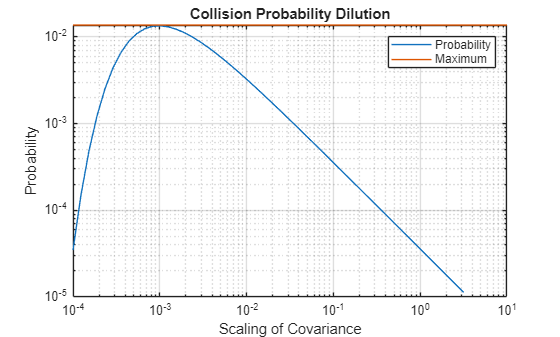
To understand the maximum verses instantaneous probability, let's plot the maximum and the instantaneous probability obtained for a fixed hard-body radius and scaling the covariance. For a very small covariance relative to the miss distance, the probability of collision is small. As the covariance increases, the probability reaches a maximum. Beyond this the probability decreases, known as dilution. This approximate formulation assumes the probability density is constant over the sphere, so we use a small value of the hard-body radius.

rSatellite = 2; % use a small value of radius for most accuracy in the comparison
[Pcmax,ksq] = maxCollisionProbability2D(conj.X_icrf(:,:,1),conj.V_icrf(:,:,1),conj.cov1_icrf,...
    conj.X_icrf(:,:,2),conj.V_icrf(:,:,2),conj.cov2_icrf,rSatellite)

Pcmax = 0.0137

ksq = 0.0019

scale = logspace(-4,0.5);
Pc0sc = zeros(size(scale));
for k = 1:length(scale)
  covC = scale(k)*(conj.cov1_icrf+conj.cov2_icrf);
  Pc0sc(k) = collisionProbability2D(conj.X_icrf(:,:,1),conj.V_icrf(:,:,1),covC,...
    conj.X_icrf(:,:,2),conj.V_icrf(:,:,2),zeros(3),rSatellite);
end
figure
loglog(scale,Pc0sc)
hold on
plot(xlim,Pcmax*[1 1])
grid on
xlabel('Scaling of Covariance')
ylabel('Probability')
title('Collision Probability Dilution')
legend('Probability','Maximum')

Impact of Avoidance Radius

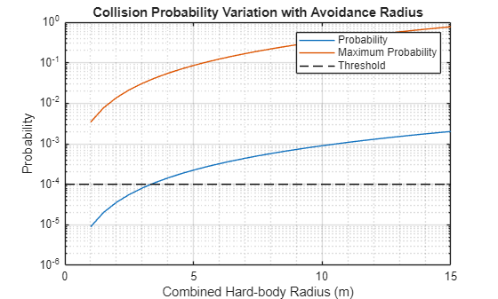
Our example has a small miss distance of 16 m. If we use a hard-body radius greater than this the probability of collision is 100%. In this code block below, we compute the probability and theoretical maximum for a range of hard-body radii below 15 m.

rSatellite = 1:0.5:15; % m
Pc0 = zeros(size(rSatellite));
Pcmax = zeros(size(rSatellite));
for k = 1:length(rSatellite)
  Pc0(k) = collisionProbability2D(conj.X_icrf(:,:,1),conj.V_icrf(:,:,1),conj.cov1_icrf,...
    conj.X_icrf(:,:,2),conj.V_icrf(:,:,2),conj.cov2_icrf,rSatellite(k));
  
  Pcmax(k) = maxCollisionProbability2D(conj.X_icrf(:,:,1),conj.V_icrf(:,:,1),conj.cov1_icrf,...
    conj.X_icrf(:,:,2),conj.V_icrf(:,:,2),conj.cov2_icrf,rSatellite(k));
end
figure('name','Collision Probability')
semilogy(rSatellite,[Pc0;Pcmax])
hold on
plot(xlim,1e-4*[1 1],'k--')
legend('Probability','Maximum Probability','Threshold')
ylabel('Probability')
xlabel('Combined Hard-body Radius (m)')
title('Collision Probability Variation with Avoidance Radius')
grid on; grid minor

Select a Probability for Comparison After the Maneuver

Let's choose a single value of the hard-body radius and resulting collision probability to compare against later, after we execute the maneuver.

conj.rSatellite =8;
conj.Pc0 = collisionProbability2D(conj.X_icrf(:,:,1),conj.V_icrf(:,:,1),conj.cov1_icrf,...
    conj.X_icrf(:,:,2),conj.V_icrf(:,:,2),conj.cov2_icrf,conj.rSatellite);
conj.Pcmax = maxCollisionProbability2D(conj.X_icrf(:,:,1),conj.V_icrf(:,:,1),conj.cov1_icrf,...
    conj.X_icrf(:,:,2),conj.V_icrf(:,:,2),conj.cov2_icrf,conj.rSatellite);

disp(table(conj.rSatellite, conj.Pc0, conj.Pcmax, ...
  VariableNames=["Hard-body radius (m)","Probability","Maximum Probability"]))

    Hard-body radius (m)    Probability    Maximum Probability
    ____________________    ___________    ___________________

             8              0.00057166           0.21877      

Maneuver Planning

Compute the Maneuver

Compute a maneuver to create separation at the conjunction time. This is a simple partial Hohmann maneuver to increase the orbit radius. Every half orbit, the satellite is at the radial maximum distance from the debris object. Due to the slight increase in mean motion, the satellite drifts relative to its original position tangentially, i.e. change phase. To return to the nominal orbit, the delta-V must be repeated in reverse after the conjunction.

The equations from [3] show how the small delta-V relates to the expected difference in tangential and radial distance achieved from the conjunction point. The radial distance is the same every orbit but the tangential distance increases with time. A similar amount of delta-V is required to return to the original orbital station, if required. Note that these equations are approximate and as real orbits have nonzero eccentricity there is always some difference in the actual change of orbit from that predicted.

$\Delta \mathit{a}\approx 2\frac{\Delta \mathit{V}}{\mathit{V}}\mathit{a}$ , $\Delta {\mathit{D}}_{\mathit{R}}=2\Delta \mathit{a}$ so that $\Delta \mathit{V}\approx \frac{\Delta {\mathit{D}}_{\mathit{R}}\mathit{V}}{4\mathit{a}}$, and $\Delta {\mathit{D}}_{\mathit{T}}\approx 3\Delta \mathit{V}\Delta \mathit{T}$

We will specify the target radial offset $\Delta {\mathit{D}}_{\mathit{R}}$. We specify the amount of time ahead of the conjunction for the maneuver using half-periods. From this $\Delta \mathit{T}$, we can predict the tangential offset $\Delta {\mathit{D}}_{\mathit{T}}$ to be achieved.

We compute the average semi-major axis $\mathit{a}$ from the mean motion $\mathit{n}$ obtained from the TLE using this formula where $\mu$ is the gravitational constant of the Earth. The mean motion $\mathit{n}=\sqrt{\mu /{\mathit{a}}^3}$ in the TLE data is in units of degrees per second, so the period is 360 times its inverse. In this code block, we compute the delta-V and predicted tangential distance from the specific radial offset and number of orbit periods. These computations are in km.

mvr.delD_R = 1.5;  % radial offset, km
mvr.nP     = 3.5; % number of orbit periods, plus 1/2
mvr.v0     = vecnorm(conj.V_icrf(:,:,1)); % m/s
mu         = 3.98600436e5; % gravitational constant, km^3/sec^2
mvr.sma    = (mu/(mission.elements(1).MeanMotion*pi/180)^2)^(1/3); % km
mvr.dVmag  = 0.25*mvr.v0*mvr.delD_R/mvr.sma; % m/s
mvr.deltaT = mvr.nP*mission.elements(1).Period;
mvr.delD_T = 3*mvr.deltaT*mvr.dVmag*1e-3;

disp(table(mvr.delD_R, mvr.dVmag, mvr.deltaT/3600, mvr.delD_T, ...
  VariableNames=["Radial Offset (km)","Delta-V (m/s)","Time Before Conjunction (hours)","Tangential Offset (km)"]))

    Radial Offset (km)    Delta-V (m/s)    Time Before Conjunction (hours)    Tangential Offset (km)
    __________________    _____________    _______________________________    ______________________

           1.5               0.41087                   5.5762                         24.744        

Next, to initialize the numerical integration, compute the states at this maneuver start time using the states() function.

mvr.mvrTime = conj.tCA - seconds(mvr.deltaT);
[mvr.X0_icrf,mvr.V0_icrf] = states(mission.sat(1),mvr.mvrTime,CoordinateFrame='inertial'); % m/s

Obtain the Satellite and Debris Ephemeris up to the Maneuver Time

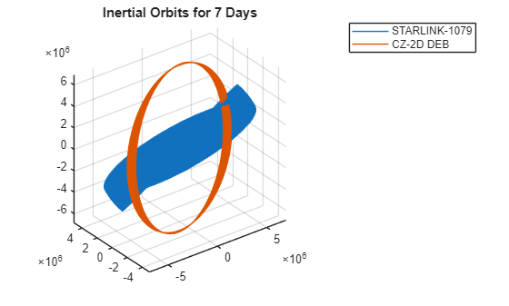
The TLE propagator is SGP4. Here we plot the orbits for the entire seven day conjunction assessment timeframe. Note, the orbits rotate in inertial space due to perturbations from the Earth and other disturbances. The StarLink satellite rotates more than the debris object.

mission.sc.StopTime = mission.startTime + nDays;
[pos_all,vel_all] = states(mission.sat,CoordinateFrame='inertial');
figure; plot3(pos_all(1,:,1),pos_all(2,:,1),pos_all(3,:,1))
axis equal
hold on
grid on
plot3(pos_all(1,:,2),pos_all(2,:,2),pos_all(3,:,2))
title(sprintf('Inertial Orbits for %d Days',nDaysDouble))
legend(mission.sat(1).Name,mission.sat(2).Name)

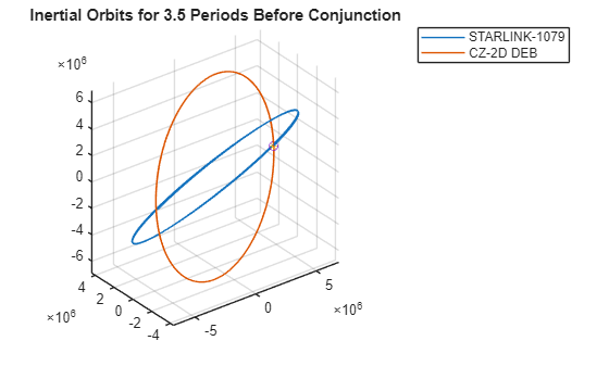
Next, plot the nominal orbits between the maneuver time and the detected conjunction.

mission.sc.StartTime = mvr.mvrTime;
mission.sc.StopTime = conj.tCA;
[pos_nom,vel_nom,t_out] = states(mission.sat,CoordinateFrame='inertial');
figure; plot3(pos_nom(1,:,1),pos_nom(2,:,1),pos_nom(3,:,1))
axis equal
hold on
grid on
plot3(pos_nom(1,:,2),pos_nom(2,:,2),pos_nom(3,:,2))
plot3(pos_nom(1,end,1),pos_nom(2,end,1),pos_nom(3,end,1),'*')
plot3(pos_nom(1,end,2),pos_nom(2,end,2),pos_nom(3,end,2),'o')
title(sprintf('Inertial Orbits for %g Periods Before Conjunction',...
  seconds(conj.tCA-mvr.mvrTime)/mission.elements(1).Period))
legend(mission.sat(1).Name,mission.sat(2).Name)

Simulate the Maneuver

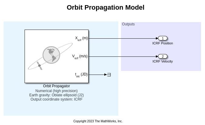
Simulate with the Orbit Propagator Block

Load the propagator model with the Orbit Propagator block. Matching SGP4 trajectories requires at least the J2 oblateness term, which defines how the Earth radius is largest at the equator and smallest at the poles. SPG4 uses the zonal only terms of J3 and J4 and no higher order terms. SGP4 include the average effect of drag but with a simple exponential model of the atmosphere. The StarLink satellite has a negative ballistic coefficient, which in this case indicates that drag has very little effect, presumably due to the satellites performing near-continuous drag makeup. First, we open the model.

mvr.mdl = "OrbitPropagationModel";
open_system(mvr.mdl);
mvr.blk = mvr.mdl + "/Orbit Propagator";

The maneuver delta-V is applied along the velocity unit vector, $$\underset{}{\overset{ˆ}{v}}$$, computed using the velocity magnitude.

mvr.vHat = mvr.V0_icrf/vecnorm(mvr.V0_icrf); % velocity direction

We simulate both the unperturbed trajectory and the trajectory with the maneuver.

X_sim = [mvr.X0_icrf mvr.X0_icrf]';
V_sim = [mvr.V0_icrf mvr.V0_icrf+mvr.dVmag*mvr.vHat]';

Set the block and model parameters with set_param().

• We specify the Julian date to significant digits, with a second input to num2str.

• Add the delta-V to the state obtained from the TLE elements and passed to inertialVelocity.

• Set the stop time on the model using the time between the maneuver and the predicted conjunction. We use a fixed step size to compare the numerically propagated trajectory both with and without the maneuver, i.e. so that the timesteps are the same for both.

set_param(mvr.blk, ...
    startDate = num2str(juliandate(mvr.mvrTime),15), ...
    stateFormatNum = "ICRF state vector", ...
    inertialPosition = mat2str(X_sim), ...
    inertialVelocity = mat2str(V_sim), ...
    gravityModel = "Oblate ellipsoid (J2)", ...
    units = "Metric (m/s)", ...
    outportFrame = "ICRF");
set_param(mvr.mdl, ...
    SolverType = "Variable-step", ...
    MaxStep = "20", ...
    RelTol = "1e-12", ...
    AbsTol = "1e-14", ...
    StopTime = string(mvr.deltaT), ...
    SaveOutput = "on", ...
    OutputSaveName = "yout", ...
    SaveFormat = "Dataset", ...
    DatasetSignalFormat = "timetable");

Simulate the trajectory after the maneuver by calling the sim function on the model.

tic
simOutput = sim(mvr.mdl);
toc

Elapsed time is 5.538485 seconds.

Check the Achieved Offset

To compute the new probability and miss distance, get the values from the output timetable.

ephPosICRF = simOutput.yout{1}.Values; % data is n×2×3
ephVelICRF = simOutput.yout{2}.Values;

no_mvr.X_icrf = squeeze(ephPosICRF.Data(:,1,:))';
no_mvr.V_icrf = squeeze(ephVelICRF.Data(:,1,:))';
no_mvr.XF_icrf = no_mvr.X_icrf(:,end);
no_mvr.VF_icrf = no_mvr.V_icrf(:,end);
mvr.X_icrf = squeeze(ephPosICRF.Data(:,2,:))';
mvr.V_icrf = squeeze(ephVelICRF.Data(:,2,:))';
mvr.XF_icrf = mvr.X_icrf(:,end);
mvr.VF_icrf = no_mvr.V_icrf(:,end);

Let's compare this simulation, before the maneuver, with the previously computed TLE-generated orbit positions at the conjunction, stored in conj.X_icrf. The results should be within 1 km, and are in fact less than 100 m.

deltaTLE = vecnorm(no_mvr.XF_icrf - conj.X_icrf(:,:,2)) % m

deltaTLE = 78.0265

Now let's compute the new distance achieved with the maneuver. We compute the distance between the endpoint of the simulation and the states at conjunction of both the satellite and the debris objects. In this case, our miss distance is very close to that predicted.

dMiss_self = vecnorm(mvr.XF_icrf - conj.X_icrf(:,:,1));
dMiss_debris = vecnorm(mvr.XF_icrf - conj.X_icrf(:,:,2));
disp(table(dMiss_self*1e-3, dMiss_debris*1e-3, sqrt(mvr.delD_R^2+mvr.delD_T^2), ...
  VariableNames=["Actual distance - self (km)","Miss distance - debris (km)","Predicted miss distance (km)"]))

    Actual distance - self (km)    Miss distance - debris (km)    Predicted miss distance (km)
    ___________________________    ___________________________    ____________________________

              24.777                         24.761                          24.789           

For visualization, we also retrieve the debris state from its TLE for the time vector output from the simulation.

mission.sc.StartTime = mission.startTime;
mission.sc.StopTime = mission.startTime+days(7);
pos_debris = zeros(3,length(ephPosICRF.Time));
vel_debris = zeros(3,length(ephPosICRF.Time));
for k = 1:length(ephPosICRF.Time)
  [pos_debris(:,k),vel_debris(:,k)] = states(mission.sat(2),ephPosICRF.Time(k)+mvr.mvrTime,CoordinateFrame='inertial');
end

Confirm the Collision Probability is Reduced

Check the new probability using maxCollisionProbability2D. Object 2's covariance is not changed. Object 1, the StarLink satellite, now has a different position so we should recompute the inertial covariance since the encounter frame has changed.

A = dcmicrf2lvlh(mvr.XF_icrf,mvr.VF_icrf);
mvr.cov1_icrf = A'*c0_lvlh*A; % convert LVLH covariance to inertial frame

The new probability is effectively zero, while the maximum probability is reduced to less than 1e-7 (depending on the hard-body radius selected above).

mvr.Pc = collisionProbability2D(mvr.XF_icrf,mvr.VF_icrf,mvr.cov1_icrf,...
  conj.X_icrf(:,:,2),conj.V_icrf(:,:,2),conj.cov2_icrf,conj.rSatellite);
mvr.Pcmax = maxCollisionProbability2D(mvr.XF_icrf,mvr.VF_icrf,mvr.cov1_icrf,...
  conj.X_icrf(:,:,2),conj.V_icrf(:,:,2),conj.cov2_icrf,conj.rSatellite);
disp(table( conj.Pc0, mvr.Pc, mvr.Pcmax, ...
  VariableNames=["Original Probability","New Probability",'New Max Probability']))

    Original Probability    New Probability    New Max Probability
    ____________________    _______________    ___________________

         0.00057166                0               1.0442e-07     

Using the rotation to the LVLH frame, we can check the miss distance in each direction. The cross-track or orbit normal direction offset is small but not nonzero because the orbits are not perfectly circular and the orbit perturbations.

dX_LVLH = A*(mvr.XF_icrf - conj.X_icrf(:,:,2));
disp(table( dX_LVLH(1)*1e-3, dX_LVLH(2)*1e-3, dX_LVLH(3)*1e-3, ...
  VariableNames=["Radial offset (km)","Along-Track Offset","Cross-Track Offset"]))

    Radial offset (km)    Along-Track Offset    Cross-Track Offset
    __________________    __________________    __________________

          1.4578               -24.718              0.0069499     

Visualize the Maneuver Results

View in a Scenario

View the results in the scenario viewer. First, create a new scenario object associated with the maneuver:

mvr.sc = satelliteScenario;

Update the ephemeris start time with the datetime for loading it back into the satellite scenario. Create timetables for the debris object ephemeris obtained from the prior scenario's SGP4 propagator. Then, pass the scenario object to the viewer function to view the orbits.

starlinkPos = ephPosICRF;
starlinkPos.Data = mvr.X_icrf';
starlinkPos.Properties.StartTime = mvr.mvrTime;
starlinkPos.Time.TimeZone = "UTC";
starlinkVel = ephVelICRF;
starlinkVel.Data = mvr.V_icrf';
starlinkVel.Properties.StartTime = mvr.mvrTime;
starlinkVel.Time.TimeZone = "UTC";

sat_n = satellite(mvr.sc, starlinkPos, starlinkVel, ...
    "CoordinateFrame", "inertial","Name","Satellite");

debrisPos = timetable(starlinkPos.Time,pos_debris'); % debris TLE position
debrisVel = timetable(starlinkPos.Time,vel_debris');

sat_d = satellite(mvr.sc, debrisPos, debrisVel, ...
    "CoordinateFrame", "inertial","Name","Debris");
sat_d.MarkerColor = [1 0.059 1];
sat_d.Orbit.LineColor = [1 0.059 1];

viewer = satelliteScenarioViewer(mvr.sc,"CurrentTime",mvr.sc.StopTime-days(5/1440));
camheight(viewer, 9.90e+06);

These screenshots, of the scenario, show that we have achieved an offset of our active satellites at the time when the debris is at its closest to the satellite orbit.

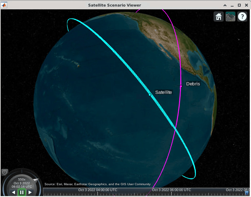
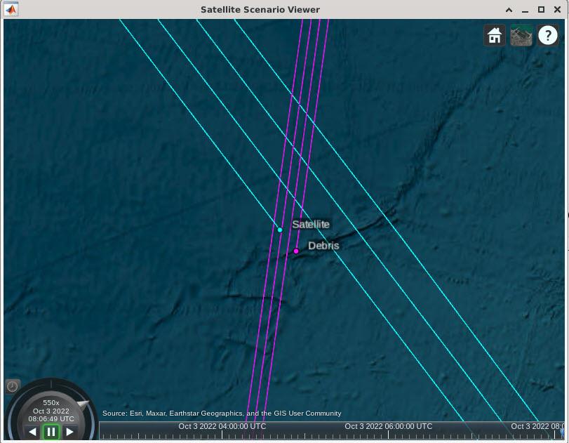
viewerZoom = satelliteScenarioViewer(mvr.sc,"CurrentTime",mvr.sc.StopTime);
camheight(viewerZoom, 1.0e+06);

This zoomed-in view at the end of the trajectories, which is the previous time of closest approach, shows that the satellite now lags the debris.

Relative State Plot

To view the relative state, we must rotate the difference in the states at every timestep. We do this in a loop for our two sets of timetables, the simulated data with and without the maneuver. We achieve a plot very similar to that of the reference [3].

xH = zeros(3,size(ephPosICRF,1));
for k = 1:size(ephPosICRF,1)
  r = no_mvr.X_icrf(:,k); % no maneuver
  v = no_mvr.V_icrf(:,k);
  A = dcmicrf2lvlh( r, v );  % Inertial to LVLH frame (RSW)
  xH(:,k) = A*(mvr.X_icrf(:,k) - r);
end
figure
plot(xH(1,:),xH(2,:))
grid on
grid minor
title('Relative State, Maneuver vs. No Maneuver')
xlabel('X in B-plane (radial) [m]')
ylabel('Y in B-plane (tangential) [m]')

We can plot the combined covariance by transforming the inertial covariances into the LVLH frame of the maneuvering satellite. To calculate the semi-major axes and rotation of the ellipse from the covariance, use the singular value decomposition with svd(). We plot the 1 and 2-sigma ellipses here.

theta = linspace(0,2*pi);
A = dcmicrf2lvlh( mvr.X0_icrf, mvr.V0_icrf );
covSum = mvr.cov1_icrf+conj.cov2_icrf;
P_lvlh = A*covSum*A';
[u,s] = svd(P_lvlh(1:2,1:2));
sma_cov = sqrt(diag(s));
disp('Ellipse semi-major axes (m):')

Ellipse semi-major axes (m):

disp(sma_cov)

  373.7744
  141.4519

x = sma_cov(1)*cos(theta);
y = sma_cov(2)*sin(theta);
rE = u*[x;y];
hold on
plot(rE(1,:),rE(2,:))
plot(2*rE(1,:),2*rE(2,:))
legend('Relative State','1-sigma','2-sigma')

Note that in operational use, check the maneuver plan to make sure it does not cause any other potential conjunctions. In addition, the satellite may need to maneuver back to station. This is about the same magnitude maneuver as that executed, but needs to be planned closer to real-time to account for disturbances and maneuver errors.

References

1. NASA Spacecraft Conjunction Assessment and Collision Avoidance Best Practices Handbook, December 2020, NASA/SP-20205011318, https://nodis3.gsfc.nasa.gov/OCE_docs/OCE_50.pdf

2. Spaceflight Safety Handbook for Satellite Operators, Version 1.5, August 2020, 18th Space Control Squadron, www.space-track.org

3. Adia, S., "Conjunction Risk Assessment and Avoidance Maneuver Planning Tools." 6th International Conference on Astrodynamics Tools and Techniques, 2016. Available on ResearchGate.

4. Alfriend, K., Akella, M., Lee, D., Frisbee, J., Foster, J., Lee, D., and Wilkins, M. “Probability of Collision Error Analysis.” Space Debris Vol. 1 No. 1 (1999) pp. 21-35 Springer. DOI 10.1023/A:1010056509803