Basel II Compliance and Risk Management Analysis: Calculating Economic Capital

Economic capital (EC), the amount of capital that an organization must set aside to offset potential losses, is a key metric for many European banks and financial institutions. It is also a central requirement of Pillar 2 of the Basel II regulatory framework. While Capgemini and many of its clients view EC as the best measure of risk inherent in a portfolio, calculating EC is not a straightforward analytical exercise. Portfolios heavily weighted in a particular sector, for example, carry a significant amount of concentration risk, complicating EC analysis.

Using MATLAB^®, Capgemini has developed a process for calculating EC that takes portfolio concentration into account. The process involves four main steps:

• Gathering inputs, including information about individual loans in the portfolio
• Preprocessing the data
• Running Monte Carlo simulations to estimate portfolio loss
• Presenting the results

We chose MATLAB because its matrix-based infrastructure is ideal for organizing the kinds of data that we deal with and the operations that are applied to this data, including the linear algebra operations that are needed for calculating EC. The ability to perform Monte Carlo simulations in MATLAB gives us another key advantage when modeling EC and other kinds of risk.

Gathering Inputs

Before calculating EC for a loan portfolio, we must determine some standard risk parameters for each loan in the portfolio. These parameters, which include probability of default (PD) and loss given default (LGD), are often provided in the databases that our clients already use for Basel II compliance. To enable the calculation of concentration risk, each loan must also be assigned to a sector—for example, utilities, energy, or automotive.

Our clients store this information in data warehouses and databases from a variety of vendors. We use Database Toolbox™ to import the information into MATLAB from any ODBC/JDBC-compliant database and from data warehouses such as Teradata. If the data is provided in spreadsheets, we use a simple call to xlsread() to read it in. After importing the data into MATLAB, we clean it by computing missing values and identifying outliers.

Calculating the Correlation Matrix and Default Thresholds

Because accounting for correlation risk is a key requirement of Basel II, we must calculate a correlation matrix that reflects the way European macroeconomic sectors are linked. Based on equity return information in all these sectors derived from multiple data sources, including Bloomberg and Dow Jones Stoxx, we calculate correlations between sectors and store them in a matrix (Figure 1). The matrix is used in the Monte Carlo simulations to incorporate sector information into the likelihood of default for each loan.

Our credit risk models are based on the Merton model, in which an obligor (a loan customer) defaults when the asset return generated in the simulation falls below the Z-default threshold. Z-default is defined as the normal inverse of the PD, which ensures that, in the long run, the obligor will default as many times as is predicted by the PD.

Running Monte Carlo Simulations

We run a Monte Carlo simulation of the portfolio for up to one million different scenarios. For each scenario (or iteration), we do the following:

• Determine which loans default
• Estimate the loss for each defaulting loan
• Sum the individual loan defaults to find the portfolio loss

To identify default loans in the portfolio, a standard normally distributed random number is determined for each loan. This number depends on a random number corresponding to its sector, which is common to all loans in that sector, and an idiosyncratic random number, drawn for each loan separately. In this way, the health of the sector that the obligor belongs to influences whether this obligor defaults.

We generate the random numbers per sector using the Statistics and Machine Learning Toolbox™ mvnrnd() function. These numbers are drawn from a multivariate normal distribution that takes into account the intersector correlations (as specified in the correlation matrix). The use of the normal distribution is not a constraint. Sometimes a multivariate t distribution (a t copula) is used if the client wants to enhance the level of tail dependence (the dependence among extreme outcomes of the asset returns) in the model.

We estimate the loss for a defaulting loan by sampling from a beta distribution based on the LGD. For example, if the LGD for a loan is 15%, we set up the parameters α and β of the distribution so that individual default losses may range from 0% to 100% but in the long run the results will be 15%.

The final step of each iteration is to total the losses for all loans in the portfolio and store the results in a loss vector. When all iterations are complete, the loss vector holds the distribution of losses for the portfolio. To compute the expected loss (EL) and the EC, we use two simple MATLAB functions:

EL = mean(Loss); 
EC = prctile(Loss,99.95) – EL;

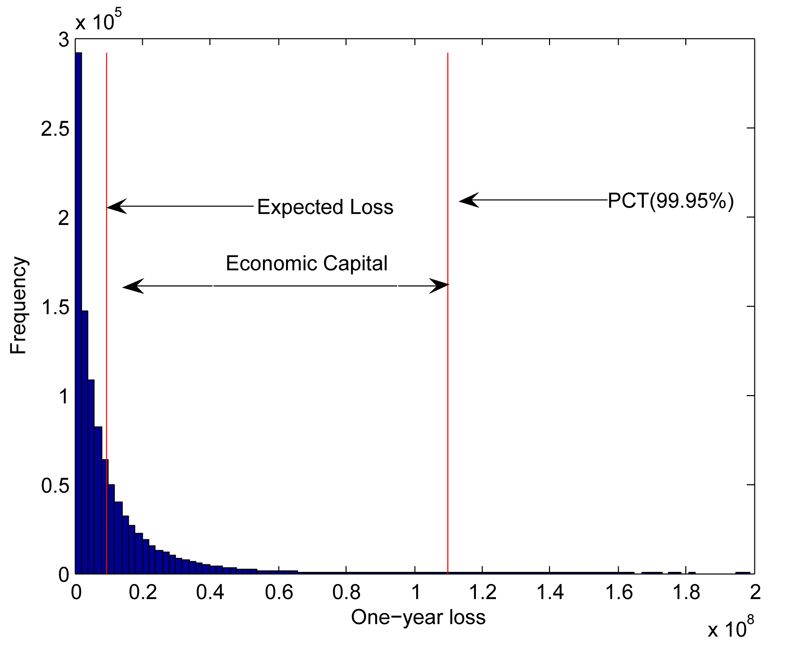
The example above calculates EC using the 99.95^th percentile, the amount of capital needed to protect the bank against losses that could occur 99.95 percent of the time. The percentile can change according to the bank’s target credit rating. Since the expected loss can also be calculated analytically, it is an ideal statistic for validating the calculations. The alignment of Monte Carlo Expected Loss with analytical Expected Loss is a standard checkpoint in our routines.

Presenting the Results

We validate and present the results to clients using a MATLAB histogram of the credit loss vector (Figure 2).

The histogram depicts the level of default correlation, enabling us to rapidly identify irregularities. If correlations are high, the histogram tends to be concentrated on the left (low losses) and right (high losses) ends of the distribution. If correlations are low, the histogram tends to be heavy in the middle of the distribution.

We use MATLAB to generate reports of the analysis, write the results to a spreadsheet, or save them in a database, depending on the client’s needs. In most cases, we provide the MATLAB source code so that the client can see how the model works and modify it for future calculations.

Many of our clients are MATLAB users. For those who are not, we use MATLAB Compiler™ to build a standalone application with a graphical user interface that lets them run sophisticated analysis and simulations without installing MATLAB.

Optimizing Performance

When running Monte Carlo simulations that require hundreds of thousands of iterations, any step that accelerates a single iteration significantly reduces simulation time. Wherever possible we use built-in MATLAB functions, which are typically much faster than those we develop ourselves. We also take advantage of MATLAB vector and matrix operations and look for opportunities to move calculations outside the simulation iterations and to eliminate nested loops. For example, many of our clients find it useful to allocate EC to each obligor. It is inefficient to use a new simulation for each obligor, so we made this an optional calculation of the main EC loop. We can then allocate EC only when we need to, and speed the calculation of overall EC when we do not.

Another example of code optimization is the declaration of vectors needed in the simulation loop with the help of a zeros or ones statement prior to starting this loop instead of using a vector that grows during the execution of the simulation loop.

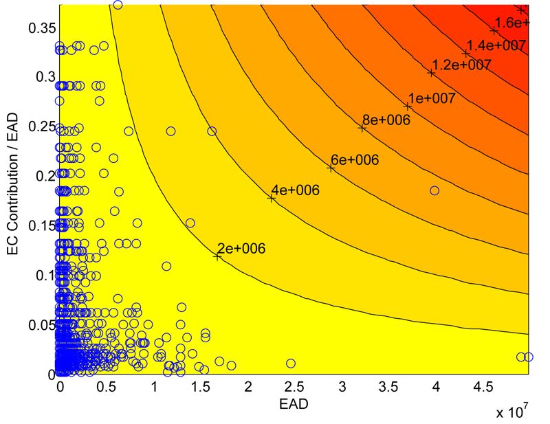
It is advisable to allocate EC to the loan level so that it is clear how much risk is generated by each loan. The results can be presented graphically for risk management purposes. For example, in Figure 3 we have plotted each loan as a circle (‘o’) on the two axes: loan size (or Exposure at Default) and risk size (or EC Contribution divided by the loan size).

Traditional risk management is concerned with monitoring large loans. This is the perspective expressed by the x-axis. With the help of the contributions, a second perspective can be added on the y-axis: the risk that each loan carries.

A Versatile Environment for Modeling Risk

We use MATLAB to model a number of other risk types. For example, we model interest rate risk in the banking book (another Pillar 2 Basel II requirement) to determine the bank’s exposure to adverse movements in interest rates. Here, instead of multivariate normal distributions, we use a t copula and generate random observations from a multivariate t distribution using mvtrnd().

We are seeing an increasing demand from rating agencies and banks for models of structured credit products, such as collateralized debt obligations and mortgage-backed securities. MATLAB helps us build and simulate exceptionally fine-grained models that take into account every instrument in a reference portfolio.