The CLASSIX Story: Developing the Same Algorithm in MATLAB and Python Simultaneously
Dr. Mike Croucher, MathWorks
Stefan Güttel, University of Manchester
CLASSIX is a fast and explainable machine learning algorithm developed by researchers at The University of Manchester. In this presentation, hear about how it was originally written in Python and then ported to MATLAB® for fun by Mike Croucher of MathWorks following an interoperability demo. Since MATLAB's profiler is more informative than anything in the Python world, this allowed the original researchers to further refine the algorithm and improve the original Python package, speeding it up by a factor of 50. Lessons from the Python package were then brought back to the MATLAB version for an additional 10x increase in speed. The work also identified a performance bottleneck in MATLAB that didn't exist in Python and provided a benchmark that allowed it to be resolved in the latest version of MATLAB. Developing the same algorithm in two environments simultaneously provided useful insights and resulted in better native Python and MATLAB packages. The MATLAB version is currently the faster of the two.
Published: 6 Nov 2024
[AUDIO LOGO]
Thanks very much. This is about the classic story, which is about how we develop the same algorithm in MATLAB and Python simultaneously. And this was really beneficial for us. So this is jointly with Mike, who is joining me here. And so before I do that, I want to briefly present to you the CLASSIX algorithm. It's a clustering method that is hopefully fast, memory efficient, conceptually very simple. It's non-iterative and deterministic and easy to tune with just two hyperparameters.
So the problem we want to solve is, we have a large number of data points in high-dimensional space, potentially, and we want to group nearby data points into the same cluster. And we want to have distinct clusters for data points that are far apart. One of the main features of CLASSIX is that it is a fully explainable method. The X in CLASSIX actually stands for explainability. And I will show you what this means in a few slides. But essentially, it actually gives a justification for the computed clusters.
We currently have three implementations, one in Python, which I would say is the most mature package available, but we also have a very good MATLAB implementation by now. And there is a kind of experimental Julia version of CLASSIX as well.
So how does CLASSIX work? So let me give you a quick example using a bunch of data points in 2D that you can see on the slide here. And our job is to assign these data points into clusters. That means we want to group nearby data points into the same cluster. And we want to have points that are distant from each other in separate clusters.
The key idea here is that we first compute the first principal component of the data. That's a very quick thing to calculate. And then we enumerate the data along that direction. So we now have the concept of a first data point, which is the leftmost data point here after projection onto the first principal axis. And then we have, of course, the second, the third data point, and so on. So we enumerate all of the data, and this now allows us to traverse the data in an ordered fashion.
So starting from the first point, what we'll do now is we will look at all the following points and compute distances, so between data point 1 and 2, between data point 1 and 3, 1 and 4, and so forth. And we will group all data points that are within a predefined radius from the first point, we will group them into a group. So you see those four points here, number 1, 2, and 4, they are data points that are within a predefined radius away from data point number 1.
Now of course, we want to perform a small number of pairwise distance calculations because this would otherwise become very expensive. But there is a small trick that we can use. We have already computed the first principal component. And it just turns out that if you project data points onto that direction, and their distance after projection is larger than the predefined radius parameter, then they must be at least radius distance apart in high-dimensional space as well.
So we can use the principal component to terminate the group search. In this example here, data point number 6 is farther away than radius from the projection of data point number 1, So data point number 6, 7, and all the following ones cannot be part of the first group. So we can discard these data points. We do not need to compute pairwise distances between data point 1 and 6, 1 and 7, and so on.
And note that there is no need for any range query data structures, like k-d trees or ball trees to implement this. This just goes linearly through the data and groups data points that are close together. We then continue with the first unassigned data point, which would be data point number 3 in this case, and group all the data points within the predefined radius into the second group.
And of course, we can use the same trick as before. So data point number 7 after projection is more than radius away from data point number 3, and therefore, it can't be part of the second group, and so neither can data point number 8, 9, and all the following ones.
So this just traverses all the data. And hopefully, the number of pairwise distance calculations remains low using this early search termination when forming the groups. We continue grouping the data. So here we go. And we have now ended up with six groups of data points, shown in color here. Now, the final step is to merge these six groups into clusters. And we do this by not looking at the whole data, but just at the starting point.
So the starting points are the special data points in each of the groups that have been assigned first. So the starting point of the first group, shown in blue, was data point number one. The first point in group number 2 was data point number 3, so that would be the second starting point, and so on.
So we will now just look at the distances of these starting points, which are kind of like a coarse representation of the overall data. And these starting points are also sorted, because they are a subset of the sorted data. So we can use the same early search termination trick in order to merge them.
And we will merge two starting points if and only if they are within 1.5 times the previous the predefined radius. So in this example here, starting point 3 and 1, they are within 1.5 times the radius parameter, so groups 1 and 2 will become part of the first cluster that we are forming. And likewise, starting point 7 shown here, which is down here, is also within 1.5 times the previous predefined radius to data point number 2, so it will also become part of the first cluster we are computing.
So these first three groups that we have computed, they now become a single cluster. And we continue doing so with all the remaining starting points and group centers. And finally, we have partitioned our data into three clusters, shown in blue, black, and yellow here. And that's the whole CLASSIX algorithm.
Notice this was a very simple procedure. There is no iteration involved. And everything is fully deterministic. Now, this means that we can actually track the algorithm as it progresses and use this retrospectively to fully explain its clustering results.
For example, if we want to understand why point number 5 and point number 8 ended up in the same cluster, we just have to remember that point number 5 was in the group that had the starting point 3. So point number 5 is within the radius distance of the starting point. And likewise, point number 8 is within radius of point number 7, which was also a starting point of a group. So we can go in small steps from point number 5 to point number 3, 7, and 8.
So in other words, there is a path that connects these data points with a path length of at most 1.5 times the predefined radius. And therefore, these two data points ended up in the same cluster. Likewise, if there is no such path between two data points, like, for example, data point 5 and 10, then these data points should be in different clusters. And in CLASSIX, we provide a function called Explain that provides textual and visual explanations for the clustering results.
And I would like to show you a quick demo of that in MATLAB. So here's MATLAB. This is a live script that you can download from the CLASSIX MATLAB GitHub repository. The problem here is that of clustering a data set that corresponds to sequences, DNA sequences of COVID viruses, and we want to identify similar strains of viruses. So that's a typical clustering problem. There is some data we have to load. It's already in memory. And all that I need to do is I'm calling the CLASSIX function with my data.
In this case, it's a matrix with about 5.7 million rows and three columns. And then I need to provide two parameters. 0.2 is the radius parameter in this case, and 500 is the minimum cluster size that we expect.
So we don't want to end up with tiny clusters that have only one or two data points. So we have this second parameter here that controls the smallest cluster that we would expect. I have just run this before the presentation on this laptop here, and it took about 12 seconds to cluster these 5.7 million data points.
And we have some ground truth labels for that. So we get fairly decent performance metrics for the computer cluster. And that's all run on a 2023 laptop. Now, we can compare this with MATLAB's DBSCAN implementation. Unfortunately, that would run out of memory when we do this on the whole data set.
So in this case, I'm only clustering 5% of the data, and that will take about eight minutes in comparison. So we are ten seconds versus eight minutes for a comparable clustering quality. So both of these give quite good clustering results.
Now, the Explain function that is available in the CLASSIX algorithm can answer questions as follows-- why did data points number 300 and 400 end up in the same cluster? So we just call explain 300 and 400, and it will then produce us the path that brings us from one of the data points to the other one. So as you can see, data point number 300 is in a group with index 210. And then there is a path from this data point, which is the group center, to the group center that will then connect to the final data point.
And if you want to see this visualized, CLASSIX automatically produces a plot like this. So this is the clustering result of the 5.7 million data points. And if you're asking if this data point and this data point here are in the same yellow cluster, CLASSIX will say, yes, this is the case, and the reason is that there is this path of data points that connect these two. So this is in MATLAB. We have an equivalent Python implementation. It's the exact same data set in Python.
This is run on a different machine. The whole data is also clustered within a fraction of maybe about ten seconds or so, I would say, gives exactly the same result as the MATLAB code. It's fully deterministic, as I mentioned. And if we compare this to HDPSCAN, which is part of sklearn, on the whole data set, that would require about 1 and a half hours to cluster, giving very similar clustering metrics, so the performance of the clustering result is comparable. But in terms of computation, time CLASSIX significantly outperforms DBSCAN and HDPSCAN.
So now. I just want to talk about how did we actually get there? And that's now, really, the tale of developing the same algorithm in two languages simultaneously. So the first or the original CLASSIX version was developed in Python with my PhD student Xinye Chen. We started in '21 and had a first archive preprint in '22 and also a GitHub release. However, this early Python version used a very inefficient disjoint set data structure, which we implemented ourselves, for keeping track of clusters.
However, we didn't really identify this as a bottleneck. And we were quite happy with the performance because we were still significantly faster than DBSCAN, for example. So here is a simple benchmark problem that we will use to illustrate the progress as this algorithm has been developed in both Python and MATLAB. It's a simple benchmark of clustering 100,000 data points in five-dimensional space.
So you see the data forms two Gaussian blobs here, and we only plot the first two components of the data. This is in Python, by the way. We do this using DBSCAN, as it's available in sklearn, the latest version of it, and also using the Python implementation of CLASSIX. So this is the old Python implementation, version, 0.8.8, that's still using the inefficient disjoint set data structure.
Now, the parameters have been tuned so that both algorithms give comparable clustering results. In fact, the run indices for both of these clusterings, DBSCAN shown on the top is near perfect, so is the one computed by CLASSIX. So the clustering in both cases is very good, but the DBSCAN runtime is about 28 seconds, whereas CLASSIX does the same job in 3.8 seconds in this case.
Yeah, so Stefan's group had a very nice clustering algorithm in Python. I work for MathWorks, and so I wanted to use this in MATLAB. And thanks to MATLAB's interoperability with Python, this turns out to be very easy to do. And so here, we show an example of creating a couple of clusters in MATLAB as MATLAB matrices, and then calling the Python CLASSIX package on it. And note that it just works. I didn't need to do any additional coding or worry about the conversion between MATLAB's matrices and NumPy arrays.
I just put py dot in front of all the CLASSIX commands, and everything just worked. And so interoperability, then, is a very simple way of bringing Python code to MATLAB. Similarly, you could run MATLAB code in Python, but that's another story, and not part of today's story. The point of all of this is that it increases the audience for the algorithm. So I've worked with the maths department at the University of Manchester for many years, and I know that there's many MATLAB users there as well as Python users.
And by using this as a demonstration, then Stefan's group could tell MATLAB users that it was very easy to use their package inside MATLAB. And we added an example of how to do this to the CLASSIX GitHub repository in Python. And I talked about this case in a presentation last year called MATLAB Meets Python, Amplifying Research Impact with Crossplatform Integration. And you'll get that link in the handout notes to this presentation.
But simply running the Python code in MATLAB wasn't enough for me. I've got a bit of a research interest in these classical clustering algorithms like this, and I really like this algorithm, and I wanted to understand it more. So I ported the Python code to MATLAB very closely as an exercise for myself to help understand the algorithm. And I sent it to Stefan and his team for comment and they took my code and ran it through the MATLAB profiler to work out where the algorithm was slow.
Yes. And of course, you can also profile code in Python. However, the MATLAB profiler is really so much better than any of the Python tools that we have seen. And it really allowed us to pin down some of the bottlenecks that are present in the code. And we identified very quickly from the MATLAB version that, indeed, we are spending a really big fraction on these disjoint set structure operations in the group merging phase.
And using this insight, we were then able to rewrite Mike's MATLAB code using another approach for the group merging. Now, MATLAB on this simple benchmark here requires about 2.3 seconds with the inefficient group merging version. However, after a very simple optimization guided by the MATLAB profiler, we were able to reduce this to about 1.7 seconds. Now, Mike's MATLAB version actually followed very closely our original Python code.
So we were then able to go back to our Python code and use a similar optimization to also achieve significant speed ups in Python.
Yep. So in summary, then, what happened here is that Stefan and his team benefited significantly from having two implementations of the same algorithm, one in Python, and one in MATLAB. It kind of allows you to look at exactly the same thing through your left eye and your right eye from very slightly different angles. And due to the MATLAB-Python interoperability, then, it was very easy for us to benchmark both codes against each other.
And MATLAB's profiler helped identify bottlenecks in both codes. So the bottom of this slide shows timing for this simple clustering benchmark run on the same machine as the codes are improving over time. And in this case, a factor of 4 is gained through the optimizations. And currently, the MATLAB implementation of CLASSIX is slightly faster than the Python version on this problem.
The precise performance implementations are, of course, the performance improvements are, of course, very problem dependent. And we have seen speedups ranging from about 1 to 40. So there are other examples where the improved codes actually are much faster than they previously were. But of course, this depends a lot on the specific data one is looking at. If you look carefully here, you will see a mention of mex.
So in fact, in the most recent MATLAB version, which is the fastest among all implementations available, we speed up a tiny part of the code using mex files. And I just want to show you a bit of detail about this. So what we do very often in CLASSIX is we need to compute vector matrix products or matrix vector products. So let's say you have a vector, A, which is a 1,000-dimensional row vector, and you want to multiply it onto a short, fat matrix, B.
So in this case, the number of rows is 1,000, so not too big, but we have maybe a million columns, because that's the number of data points that we are looking at. I can do this in MATLAB in a fraction of a second, so about 30 milliseconds. And if I now want to do a matrix vector multiplication with only half of the data in B, so I want to throw away half of the columns in B, that should, in theory, be twice as fast, because I'm only doing half the number of arithmetic operations.
However, it turns out it's actually about 7.1 times slower than computing the full vector matrix product. So we notice this again using the MATLAB profiler. And I went back to Mike and asked his opinion on that.
Yeah. And the short answer is that when you create that submatrix of B, MATLAB is literally creating it. That is, it allocates a bunch of memory for an intermediate array. Then, it copies all of the requested elements into it before finally doing the product. And what Stefan and his team were expecting was just a view into the matrix B, essentially just saying, only consider this half of the matrix when you do the product.
And so obviously, it was much slower than it needed to be. And so I took this to our core math development team and asked them if there was anything they could do about this. And there wasn't time to come up with a full solution in any reasonable time frame. But what they have done is created an internal undocumented function that's available in R2024b that works for this particular case.
And you can see that we used it m and it gives almost exactly the performance difference that we would expect. And what we're going to hopefully do is work with Stefan and other people in the community to maybe bring this to a full feature at some point in the future.
So I guess, in summary, it's fair to say that not only has MATLAB helped us as an algorithm developer to improve Python and MATLAB code, but reversely, we might have even contributed a small performance improvement to MATLAB. And this brings me to the end of our presentation. We have seen how one can very easily use a Python package from within MATLAB using interoperability.
We have seen how it can be very beneficial to rewrite a Python code in MATLAB or maybe even vice versa, and then just gain insights using, for example, the MATLAB profiler in order to improve the algorithm in multiple languages simultaneously. And perhaps MATLAB can also benefit from some of those performance improvements.
I put here a link to the GitHub repository of the CLASSIX code. It's also on file central. And there is also a reference to the CLASSIX paper. Thanks very much for your attention.
[AUDIO LOGO]