Counterparty Risk Assessment with Two Steps: Monte Carlo and Parallel Computing
Pablo García Estébanez, Banco Sabadell
In this presentation, discover a novel approach to counterparty risk assessment using a two-step process: Monte Carlo simulations and parallel computing. This method leverages Monte Carlo simulations to model and quantify risk under various scenarios, followed by parallel computing to efficiently process and analyze large datasets. Learn how this integrated approach enhances the accuracy and speed of risk assessments, enabling more robust financial decision making. See practical examples and insights drawn from extensive experience in quantitative analysis and financial modeling.
Published: 22 Oct 2024
OK. Good afternoon, everybody. I'm going to speak about counterparty risk assessment with 2-step Monte Carlo parallel computing. This is a very classical problem. Until now, it was not feasible, because the powerful of the computing that we need. But just now, with new tools, with possibility of parallel computing, is really easy to deal with. So, go on.
We are going to-- this is the index. We are going to talk what remained, what is the exposure and counterparty risk metrics. After that, we are going to speak about computational framework. Then we are going to speak about tools, a little conclusions.
So the first slide. I use that to explain what is exposure. Exposure is, in its broadest sense, is a present or a future value that present of risk of default. The present value of a deal is known, but the future is uncertain.
So the classical exposure, a lot of people, is a little reminder, is the Expected Positive Exposure, EPE. If the positive part of a value. And it gives a metrics known as CVA. That is the negative adjustment value, valuation, adjustment, valuation, because of the probability of the counterparty's default.
And then there is the expected negative exposure. It gives you the DVA, and is the positive valuation adjustment that is because of the probability of your own default. And the other exposure definition could be the potential future exposure. The potential future exposure is given counterparty's default, given it, is the maximum with a high level of-- high confidence level. Is the maximum loss you can take.
In the left side of the slide, it shows you a figure of a trade. This is a It's extra trade. And we showed you-- we saw here the MtM is the present exposure, the present value. And the thin lines are the possible-- some possible path of this value. We have simulate thousand of that. We saw some of them.
And over these possible values, we can calculate the exposure as we defined before. Here is the maximal potential exposure. They put potential future exposure with the maximum here.
Here is the expected positive exposure. The area is some quite proportional to the CVA. And in thick blue line, this line, is the speculative negative exposure. And the area is proportional to DVA. Go on.
Oh, the computational framework, the main issue is when you don't have a closed formula to-- a closed evaluation formula for a derivative. This is very common in exotic derivatives. And you have two problems. When you don't have a close formula, maybe you have to calculate the mark-to-market. And the mark-to-market is a standard problem, because if you are based on current market inputs, or you have to evaluate and simulate future scenarios in thousand of scenarios.
So for every deal and every future time, it's imperative to perform a thousand of evaluations here. For example, in these scenarios of euro-dollar exchange in this date, you have to evaluate in each scenario. You have to do the evaluation of the derivative. And the computational cost becomes unfeasible with conventional architecture tools if you don't have a closed formula.
I showed you the process. The process to compute exposure is, firstly, we simulate risk factors over the time until the time of maturity of the derivative. We simulate a lot of x scenarios, a thousand of scenarios. And in each time and each scenario-- for example, here-- you have to evaluate the derivative. So this evaluation can be with a closed formula. You are lucky in this case. Or it should be with an numerical approach.
For example, Monte Carlo. Monte Carlo, in each point here, you have to do a Monte Carlo. It could be with PDEs. So it could be with trees. Anyway.
So in each point, you have one valuation. And after the evaluation, in all scenarios of all the times, you can compute your exposure, EPE, NE, or potential future exposure. This is the problem. What we can see here, the problem is a lot of scenarios to do a lot of Monte Carlo evaluations in all the scenarios in all times. This is really, really complex problem, computational.
OK. Here I will introduce what the title of my presentation was, includes "parallel computer" term. What is parallel? The main idea for parallelization is parallel size-- these scenarios.
This scenario could be compute with one worker. This scenario could be compute with another worker, another processor, another PC on the cloud, and so on. You can parallel size the compute of the scenarios in a lot of machine resources.
So now we are going to talk about netting. Netting, what is netting? Netting is when you have several deals and you are under a collateral agreement, you can offset the valuations when they have different signal.
For example, you have a scenario of the euro-dollar. Euro-dollar, euros increase, dollar decrease. You are here in this scenario.
One deal, one month, at the money forward, is negative. Another deal with the same counterparty is positive. So the netting means that in this scenario, you can offset. You can sum up these values, the .
In this case, this is a perfect netting. So these two values are going to perfect sum zero. So if you have, in this example, these two deals, do netting like that in the first month, because they are both at the money forward. They have a perfect netting. But after that, they still remain the other field. This is always with the same counterparty and with under collateral agreement.
Now I'm going to show you a real example. This is more complex. Here is a USD-sell actual TARF with a lot of-- with something like this is one-year time to maturity. You have, I think, 24 liquidation and settlement dates. Do you know, on a TARF, you liquidate every two weeks, I think, in this example. In the downside, you have an accumulator, a fixed accumulator. And in the other sense, this is a USD-buy.
So the deal, the netting when you're netting that, is scenario, various scenario, this is very, very important. You have these kind of new scenarios for the netting. When you have the netting scenarios, you can compute your exposure. You can see here the thick lines-- black, red, blue.
And here are the results of this netting with two deals. You have the maximum potential future exposure in one deal was-- in the first deal was 216 kilo-euros. In the other, it was 215. And the netting is not the sum. It's 218.
This is here the maximum potential exposure. And this is here. And it corresponds more or less to this point, to the accumulator maximum exposure.
What we can see is here, in the middle of the year, you have a potential exposure that is around 200,000, and is not the sum of one deal, 200,000 here. And here, 150,000. Is not the sum.
There is a good netting-- not perfect netting, but the sum of the two maximal potential future exposure is bigger than the netting. So you are interested in the netting.
This is the same thing for the EPE area. So the sum is, if you are less than the sum of two. And in the area, the sum is fewer, is not-- and then the sum of two is fewer of the second one. And 4 plus 20, 32, is the half of the sum.
So from the front desk and from the distribution teams, et cetera, they ask us to do netting, netting, netting, because they are interested in a lower metric risk in a lower valuation adjustment. What's the time? OK.
So the computational complexity is very, very important. In Monte Carlo valuation, you have a first step with N1 x scenarios, and second step. In each scenario, you have a Monte Carlo with N2 simulations.
In semi-analytical valuation, you have a first step with N1 scenarios, and second step is a closed formula valuation. It's very quick, that. So the computational complexity is different. In 2-step Monte Carlo, is proportional to N1 by N2 by N deals, by N dates, is very expensive, prohibitive. And in semi-analytical is N1 by N deals by N dates.
N1 is more important in path-dependent deals, because N1 represents at a time t, it represents the past-- so the path dependence history. And one is more important when the max exposure is nearer to maturity, because in the maturity, there are no more future variants. So the N2 has no sense.
In semi-analytical approach, N2 is relevant because you have a closed formula. And in 2-step Monte Carlo, N2 is more relevant at very early times because you have all the future variance still . So this is very important.
So this was the complexity with a single deal. And the complexity with a netting set is something quite different, because with a netting set, the problem is explained here. You need all valuation in all relevant dates, all deal valuation in all relevant dates.
So when you add a deal, you have a deal, and you have there their dates there-- liquidation, settlement dates, et cetera. So the computational time will increase quadratically. So it's very complex problem at first.
When you start to repeat the dates, because when you have a big netting set, the dates of settlements can be the same between several deals, the running time will increase in a linear rate with a lot of deals. So it's good news.
So after that, you have the consideration with the computation time increase quadratically with accuracy of mean estimators, as always in Monte Carlo, so that if you want double of accuracy, you have to perform four times simulations. So this is a classical problem with Monte Carlo.
And with percentile, this is for CVA and DVA for expected exposure. For potential exposure, for percentile is different because percentile don't follow this rule. But you have to do the best analysis to understand your problem. You can use that as a start point in this rule of quadratic increase.
Well, in a semi-analytical evaluation, when you have a semi-analytical evaluation with N1 as scenario, a closed formula, is not a problem, because it's faster than 2-step Monte Carlo. So it's not the primary concern.
And with N1, a number of scenario, the computational time increases linearly at early times. But at the end of the problem, at near to maturity, it becomes a simple one step on Monte Carlo problem, and it increase quadratically.
And hybrid approach is the more interesting. It combines the two kinds of OPS of deals. And, well, is really determined by set, but by the first kind of deal, by full 2-step Monte Carlo evaluation, because the semi-analytical valuation is very quick. It's really, really .
We are going to talk about tools. This is a slide borrow from MATLAB. This is the source.
The tools is the Parallel Computing Toolbox and the Parallel Server Toolbox. Well, we have used, for this example, only with the Parallel Computing Toolbox and with the cores of one single PC, desktop PC. With 12 cores-- I use 12 cores.
And, well, what I want to say is you have one instruction, parfor, that replace the for loop, the classical for loop. Is very simple.
You have to follow some rules to use that. You can't have dependency in the variables. Some rules.
But it's quite useful, this kind of instruction. Very simple to use. And it can scale your computation, parallel size your computation in multiple-core CPUs, in GPUs, and with 1/8 of the Parallel Server, in cluster of PCs, in cluster in the cloud, et cetera, et cetera.
So it's very simple to use parfor. parfor, it parallel size the loop, a classical loop for. There are a lot of other instructions about parallelization. But I think this is the more easy to start with. And for our problem is really the more interesting.
The second slide. This is an example of Monte Carlo. This is not the same kind of problem. But this is a Monte Carlo simulation.
You can see the for loop, MATLAB for loop, replaced by the parfor MATLAB loop. The other lines, code lines, are exactly the same.
And you have 30 workers. OK? 30 workers. 30 computational units.
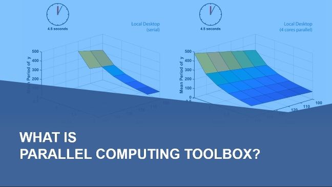
In this case, you pass from 60 seconds of running time to almost four seconds of running times. You have a gain of 15. You are 15 times faster.
You have 30 workers. You have the-- OK. As you can see, the asymptotic gain would be 30. In theoretical, you don't have the theoretical, because for parallel sized, you have to do some task. MATLAB do for you some task. But this is a good gain.
In my problem, in my tool, the gain is around the same. We have 12 cores and we have a gain of 6. And if we scale, we expect some kind of rate.
So on. Go. So we are going to conclude.
The traditional approach for counterparty risk is based on simplified models. There are some nice models, analytical models, for the simple case. The Brigo's formula is very well known for quants. But they don't fit well in a general framework of netting.
Now, the increase of computational power allows us to address the problem in a universal way without such approximation. I insist on the simplest way for our problem is to reduce the running time parallelization in scenarios across the available workers. In our case, worker are cores, but it could be other PCs. It could be GPUs. It could be a PC cluster, et cetera.
But this is really transparent for you. You put one-- you define your power pool. And after that, you replace your for by parfor. This is transparent.
Nevertheless, it's not so easy. You have to do a big effort on architecture and computer optimization, keeping basic math operation and memory transfer to a minimum. Is max with a smart selection of simulate dates. This is very important.
You have to dynamic map in one, scenarios, and in two, Monte Carlo, in regards to metric and meter error and deals of the netting set.
And finally, you must do a set to evaluate the variance of your metric. It could be running a lot of times one problem and doing histograms, Monte Carlo histograms, et cetera. You can build an external process to estimate your variance-- what is the accuracy of your estimator or your metric.
And the second part of the conclusion, we insist this very-- develop and optimize your architecture first with a classical for loop with a small number of simulations. And after that, when all works, change to parfor and optimize the bag a little bit. But it's not very complicated.
The second thing is try different parallelism method. It's really easy to change with MATLAB, with the Toolbox. There are a lot of interesting infos about parallelization task, about you have the tool too.
Choose your parallelization methods. First versus process is quite different, is the way you share the memory. You put your processing in the processor, in the cores.
You consider GPUs arise. This is for GPUs. And choose between CPU and GPU.
Here I want to say GPU is not always the best option. It depends on the problem. You have to minimize the memory transfer. So there are some problems that this is not very, very effective.
For example, for the problem I've shown, we think a CPU processor is better than GPUs. We have tests, and we have conclude this thing.
So thank you for your attention.