Dynamic Bandwidth Channel Access in Wi-Fi Networks using Wireless Network Modeler App

Since R2026a

Dynamic bandwidth channel access (DBCA) enhances spectrum efficiency by automatically adjusting the channel bandwidth in response to network conditions and requirements. This example demonstrates how to use the Wireless Network Modeler app to configure and simulate dynamic bandwidth channel access (DBCA) in a Wi-Fi® scenario with two basic service sets (BSSs). In this example, you create two BSSs, each with a Wi-Fi access point (AP) and station (STA), configure their channels and bidirectional traffic, add a TGax fading channel model, and run the simulation. The results include state transition plots and throughput calculations for each BSS. For more information about DBCA, see Dynamic Bandwidth Channel Access in Wi-Fi Networks.

First, you must create a Wi-Fi network containing two BSSs, each consisting of a Wi-Fi AP and an STA, in the Wireless Network Modeler app.

Create Wi-Fi Network

Create a network by following these steps.

1. Open the Wireless Network Modeler app.

   • MATLAB Toolstrip: On the Apps tab, under Wireless Communications, click the app icon

   • MATLAB Command Prompt: Enter wirelessNetworkModeler

2. On the app toolstrip, click New Session and select WLAN Network.

3. In the Scenario Canvas Layout section of the dialog box, set Length (m) to 50 and Breadth (m) to 50.

4. In the Nodes Placement section, set Number of APs to 2 and Number of STAs per AP to 1.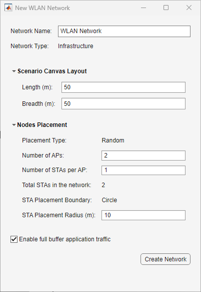

   

5. Verify that you have selected Enable full buffer application data traffic.

6. Click Create Network.

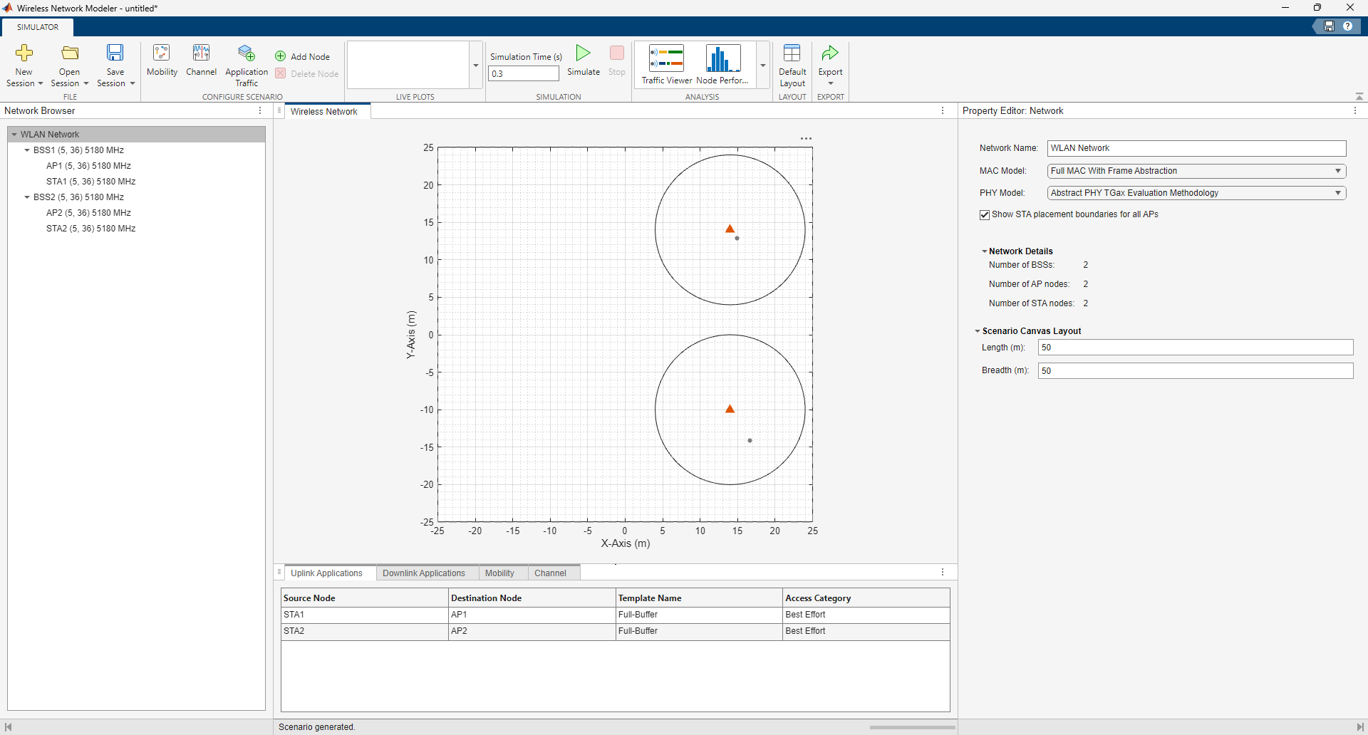
Select MAC and PHY Models

To select the medium access layer (MAC) model and physical layer (PHY) model, in the Property Editor: Network pane, set MAC Model to Full MAC and PHY Model to Full PHY.

Configure BSS1

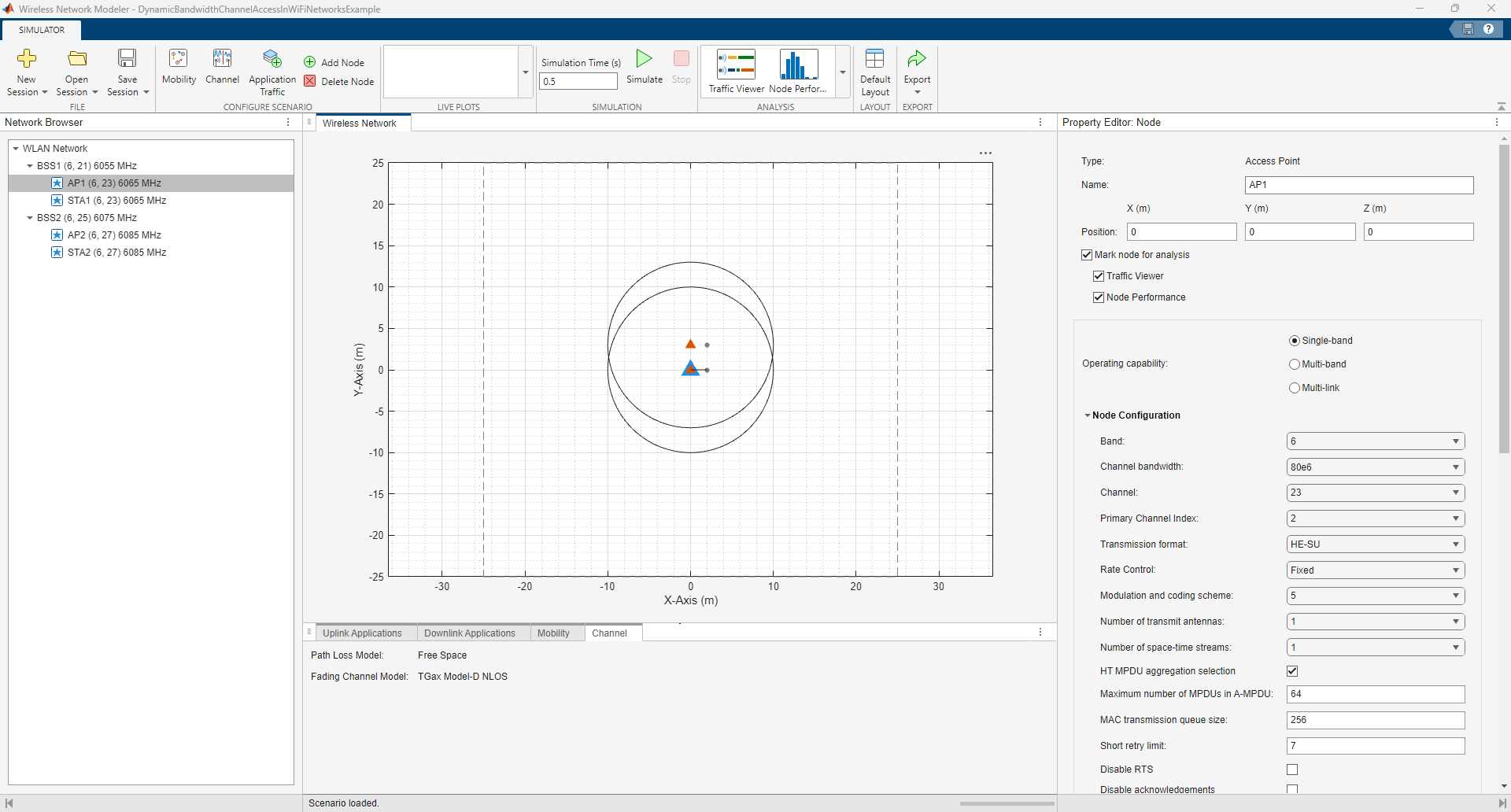
Configure BSS1, which consists of an AP and an STA operating in the 6 GHz frequency band on channel 23 with a channel bandwidth of 80 MHz. Set the primary 20 MHz channel of BSS1 to channel 21. Follow these steps to configure BSS1.

1. In the Network Browser pane under BSS1, select AP1. In the Property Editor: Node pane for AP1, set Position of AP1 by specifying the coordinates in meters: X (m) as 0, Y (m) as 0, and Z (m) as 0.

2. In the Property Editor: Node pane for AP1, in the Node Configuration section, specify these fields.

   • Band — 6

   • Channel bandwidth — 80e6

   • Channel — 23

   • Primary Channel Index — 2

   • Modulation and coding scheme — 5

   • Interference modeling — Overlapping adjacent channel

   Note that the value of Primary Channel Index sets the primary 20 MHz channel of BSS1 to the second 20 MHz channel, channel 21.

3. By default, the app applies Access Category Configuration for the AP to its associated STAs as well.

4. Click Apply. Confirm the new values for band, channel, and channel center frequency for BSS1, AP1, and STA1 in the Network Browser pane.

5. In the Network Browser pane under BSS1, select STA1. In the Property Editor: Node pane for STA1, set Position of STA1 by specifying the coordinates in meters: X (m) as 2, Y( m) as 0, and Z (m) as 0.

6. In the Property Editor: Node pane for STA1, in the Node Configuration section, specify these parameters.

   • Modulation and coding scheme — 5

   • Interference modeling — Overlapping adjacent channel

7. Click Apply.

Configure BSS2

Configure BSS2, which consists of an AP and an STA operating in the 6 GHz frequency band on channel 27 with a channel bandwidth of 40 MHz. Set the primary 20 MHz channel of BSS2 to channel 25. Follow these steps to configure BSS2.

1. In the Network Browser pane, select AP2. In the Property Editor: Node pane for AP2, set Position of AP2 by specifying the coordinates in meters: X(m) as 0, Y(m) as 3, and Z(m) as 0.

2. In the Property Editor: Node pane for AP2, in the Node Configuration section, specify these parameters.

   • Band — 6

   • Channel bandwidth — 40e6

   • Channel — 27

   • Primary Channel Index — 1

   • Modulation and coding scheme — 5

   • Interference modeling — Overlapping adjacent channel

3. Verify that Apply to all associated STAs is selected, under Access category configurations. This setting applies the access category configurations of this AP to all associated STAs.

4. Click Apply.

5. In the Property Editor: Node pane for STA2, set Position of STA2 by specifying the coordinates in meters: X (m) as 2, Y (m) as 3, and Z (m) as 0.

6. In the Property Editor: Node pane for STA2, in the Node Configuration section, specify these parameters.

   • Modulation and coding scheme — 5

   • Interference modeling — Overlapping adjacent channel

7. Click Apply.

Configure Channel

By default, the app uses TGax Model-D NLOS as the fading channel model. This example retains the default channel model.

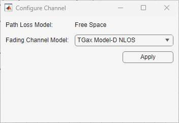
You can exclude fading effects and use only free-space path loss. In the Configure Scenario section of the toolstrip, select Channel, and in the Configure Channel dialog box, set Fading Channel Model to None. Click Apply.

Configure Application Traffic

During network creation, this example enables full buffer application data traffic. This configures both uplink and downlink full buffer application traffic between AP1 and STA1, and between AP2 and STA2.

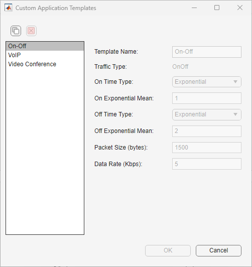
You can also change the application traffic. In the Configure Scenario section of the Application Traffic toolstrip, select Application Traffic. Then, in the Customize section of the app toolstrip and click Application Templates. In the Custom Application Templates dialog box,select your preferred traffic type from the left pane, and click to create a custom traffic template that uses the selected traffic type as a base. Finally, click OK.

In the Select uplink node pair(s) pane, choose the uplink nodes in the network to which you want to apply your application template. In the Select and apply templates pane, set Application Template and Access Category as needed, then click Apply. Next, select Downlink Application select and in the Select downlink node pair(s) pane, select the downlink nodes. Again, set the Application Template and Access Category as required, and click Apply. Finally, click Accept on the toolstrip to apply your changes or Cancel to discard them, and return to the Modeler tab of the app toolstrip.

Note that, by default, the app sets Access Category to Best Effort.

Simulate and Analyze Network Performance

In the Network Browser pane, select AP1. In the Property Editor: Node pane for AP1, select Mark node for analysis. Repeat this process for AP2, STA1, and STA2.

In the app toolstrip, in the Simulation section, click Simulate. You can monitor progress using the status bar at the bottom of the window.

Once the simulation is complete, you can analyze the throughput, latency, and packet loss of the nodes. In the Analysis section of the app toolstrip, select Node Performance to display the Node Performance pane.

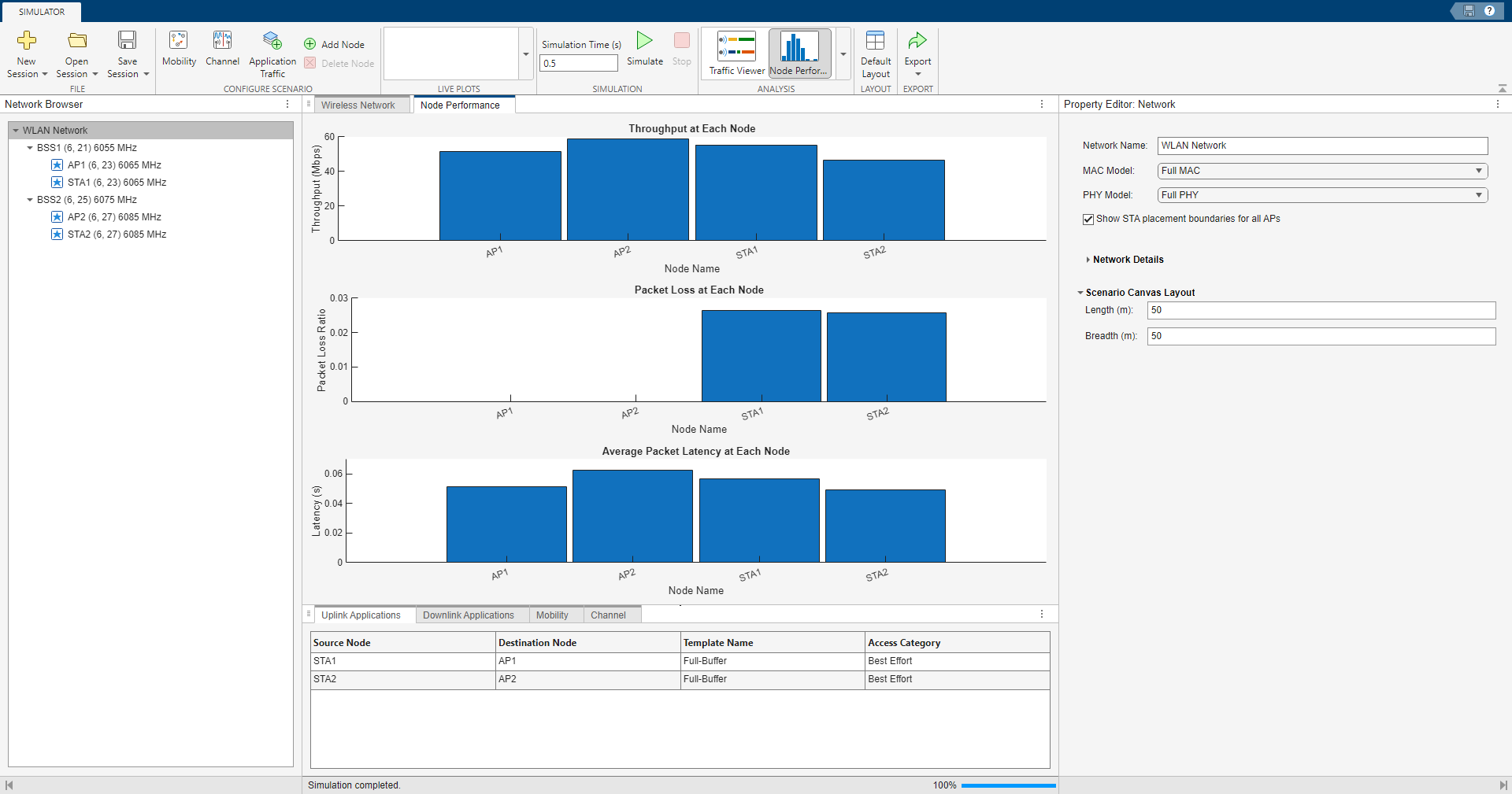
This table summarizes the key performance indicators observed in the figure.

Key performance indicators	AP1	STA1	AP2	STA2
Throughput (Mbps)	51.720	55.392	58.752	46.512
Packet loss ratio	N/A	0.026	N/A	0.026
Latency (seconds)	0.051	0.056	0.063	0.049

To view the state transitions and channel occupancy of the WLAN nodes, in the Analysis section, select Traffic Viewer. The Wireless Traffic Viewer window provides a visual summary of how each node transitions between the contend, transmit, receive, listen, and sleep states. The channel occupancy plot shows exactly which frequencies the WLAN occupies at each moment within the configured 6 GHz band.

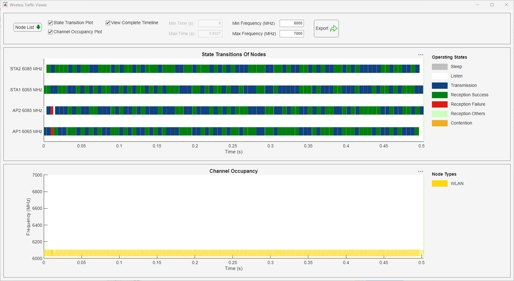
The Wireless Traffic Viewer shows that transmissions Transmissions in BSS1 and BSS2 overlap, as BSS1 uses the primary 40 MHz out of the 80 MHz available for channel 23 and BSS2 uses the secondary 40 MHz channel.